

 Download PDF
DATASHEET SEARCH SITE
Document overview
- PDF pages: 9
Technical content
Page 1
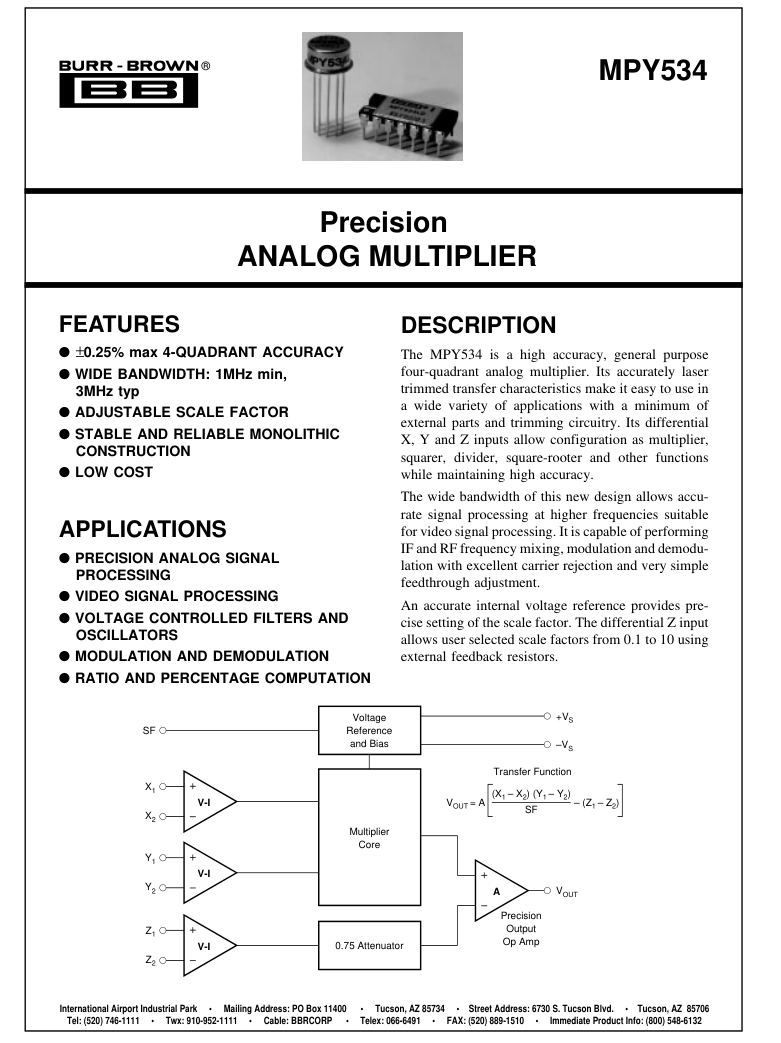
©1985 Burr-Brown Corporation
PDS-614D
Printed in U.S.A. October, 1993
SBFS016
Page 2
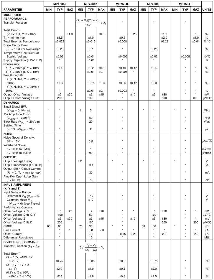
SPECIFICATIONS
ELECTRICAL
TA = +25°C and VS = ±15VDC, unless otherwise specified.
Page 3
SPECIFICATIONS (CONT)
ELECTRICAL
TA = +25°C and VS = ±15VDC, unless otherwise specified.
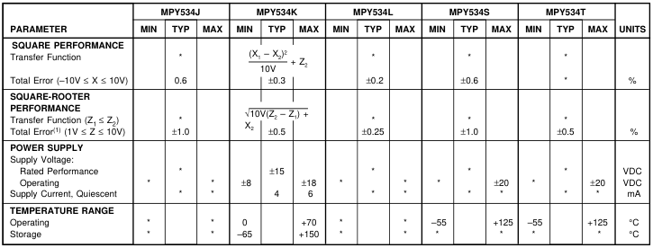
\*Specifications same as for MPY534K. NOTES: (1) Figures given are percent of full scale, ±10V (i.e., 0.01% = 1mV). (2) May be reduced to 3V using external resistor between –Vs and SF. (3) Irreducible component due to nonlinearity; excludes effect of offsets.
PIN CONFIGURATIONS
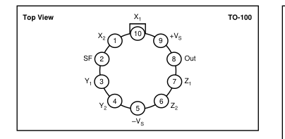
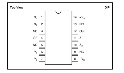
ABSOLUTE MAXIMUM RATINGS
| PARAMETER | MPY534J, K, L | MPY534S, T |
|---|---|---|
| Power Supply Voltage Power Dissipation Output Short-Circuit to Ground Input Voltage (all X, Y and Z) Operating Temperature Range Storage Temperature Range Lead Temperature (soldering, 10s) | ±18 500mW Indefinite ±V S 0°C to +70°C –65°C to +150°C +300°C | ±20 * * * –55°C to +125°C * * |
ORDERING INFORMATION
| MODEL | PACKAGE | TEMPERATURE RANGE |
| MPY534JD MPY534JH MPY534KD MPY534KH MPY534LD MPY534LH MPY534SD MPY534SH MPY534TD MPY534TH | Ceramic DIP Metal TO-100 Ceramic DIP Metal TO-100 Ceramic DIP Metal TO-100 Ceramic DIP Metal TO-100 Ceramic DIP Metal TO-100 | 0°C to +70°C 0°C to +70°C 0°C to +70°C 0°C to +70°C 0°C to +70°C 0°C to +70°C –55°C to +125°C –55°C to +125°C –55°C to +125°C –55°C to +125°C |
\*Specification same as for MPY534K.
PACKAGE INFORMATION
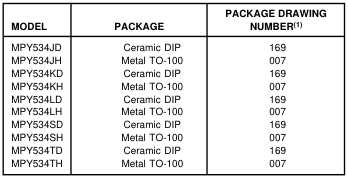
NOTE: (1) For detailed drawing and dimension table, please see end of data sheet, or Appendix D of Burr-Brown IC Data Book.
Page 4
DICE INFORMATION
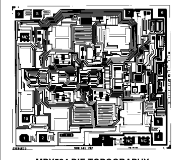
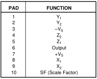

| MILS (0.001") | MILLIMETERS | |
| Die Size Die Thickness Min. Pad Size | 100 x 92 ±5 20 ±3 4 x 4 | 2.54 x 2.34 ±0.13 0.51 ±0.08 0.10 x 0.10 |
| Backing Gold | ||

TYPICAL PERFORMANCE CURVES
TA = +25°C, VS = ±15VDC, unless otherwise noted.
AC FEEDTHROUGH vs FREQUENCY
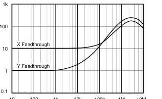
10k
10 100 1k
100k 1M 10M
Frequency (Hz)
COMMON-MODE REJECTION RATIO vs FREQUENCY
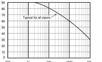
10k 1k
100k 1M
Frequency (Hz)
BIAS CURRENTS vs TEMPERATURE (X,Y or Z Inputs)
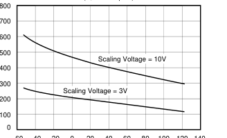
–20 0 20 40 60 80 100 120 140 –60 –40
Temperature (°C)
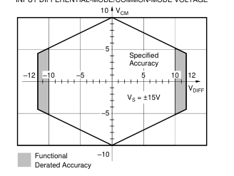
INPUT DIFFERENTIAL-MODE/COMMON-MODE VOLTAGE
Page 5
TYPICAL PERFORMANCE CURVES (CONT)
TA = +25°C, ±VCC = 15VDC, unless otherwise noted.
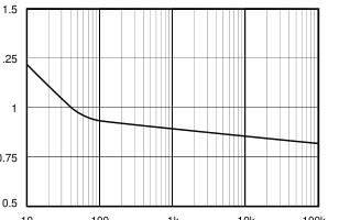
NOISE SPECTRAL DENSITY vs FREQUENCY
1k
10 100
10k 100k
Frequency (Hz)
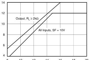
INPUT/OUTPUT SIGNAL RANGE vs SUPPLY VOLTAGES
8 10 12 14 16 18 20
Positive or Negative Supply (V)
THEORY OF OPERATION
The transfer function for the MPY534 is:
(X1 – X2) (Y1 – Y2)
VOUT = A – (Z1 – Z2)
SF
where: A = Open-loop gain of the output amplifier (typically 85dB at DC). SF = Scale Factor. Laser-trimmed to 10V but adjustable over a 3V to 10V range using external resistor. X, Y, A are input voltages. Full-scale input voltage is equal to the selected SF. (Max input voltage = ±1.25 SF.) An intuitive understanding of transfer function can be gained by analogy to an op amp. By assuming that the open-loop gain, A, of the output amplifier is infinite, inspection of the transfer function reveals that any VOUT can be created with an infinitesimally small quantity within the brackets. Then,
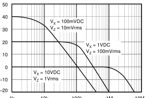
FREQUENCY RESPONSE vs DIVIDER DENOMINATOR INPUT VOLTAGE
1k 10k
1M 10M
100k Frequency (Hz)
FREQUENCY RESPONSE AS A MULTIPLIER 10
| 0 | d | B = 0.1Vr | ms; | R | L | = 2 | kΩ | C L | = 1 | 0 | 00pF | ||||
| C L | ≤ | 1 | 000pF | C L | = | 0p | F | ||||||||
| C F | = | 0 | pF | C ≤ L C ≤ F | 1000p 200pF | F | |||||||||
| A | Wit Fee tte | h db nu | X a a | 10 ck tor | C | No on | rm ne | al ction |
0
–10
–20
–30 10k
100k
1M
10M
Frequency (Hz)
an application circuit can be analyzed by assigning circuit voltages for all X, Y and Z inputs and setting the bracketed quantity equal to zero. For example, the basic multiplier connection in Figure 1, Z1 = VOUT and Z2 = 0. The quantity within the brackets then reduces to: (X1 – X2) (Y1 – Y2) – (VOUT – 0) = 0
SF
This approach leads to a simple relationship which can be solved for VOUT. The scale factor is accurately factory-adjusted to 10V and is typically accurate to within 0.1% or less. The scale factor may be adjusted by connecting a resistor or potentiometer between pin SF and the –VS power supply. The value of the external resistor can be approximated by:
SF
RSF = 5.4kΩ
10 – SF
Page 6
Internal device tolerances make this relationship accurate to within approximately 25%. Some applications can benefit from reduction of the SF by this technique. The reduced input bias current and drift achieved by this technique can be likened to operating the input circuitry in a higher gain, thus reducing output contributions to these effects. Adjustment of the scale factor does not affect bandwidth. The MPY534 is fully characterized at VS = ±15V, but operation is possible down to ±8V with an attendant reduction of input and output range capability. Operation at voltages greater than ±15V allows greater output swing to be achieved by using an output feedback attenuator (Figure
2).
BASIC MULTIPLIER CONNECTION
Figure 1 shows the basic connection as a multiplier. Accuracy is fully specified without any additional user trimming circuitry. Some applications can benefit from trimming one or more of the inputs. The fully differential inputs facilitate referencing the input quantities to the source voltage common terminal for maximum accuracy. They also allow use of simple offset voltage trimming circuitry as shown on the X input. The differential Z input allows an offset to be summed in VOUT. In basic multiplier operation, the Z2 input serves as the output voltage reference and should be connected to the ground reference of the driven system for maximum accuracy.
A method of changing (lowering) SF by connecting to the SF pin was discussed previously. Figure 2 shows another method of changing the effective SF of the overall circuit using an attenuator in the feedback connection to Z1. This method puts the output amplifier in a higher gain and is thus accompanied by a reduction in bandwidth and an increase in output offset voltage. The larger output offset may be reduced by applying a trimming voltage to the high impedance input Z2. The flexibility of the differential Z inputs allows direct conversion of the output quantity to a current. Figure 3 shows the output voltage differentially-sensed across a se- ries resistor forcing an output-controlled current. Addition
of a capacitor load then creates a time integration function useful in a variety of applications such as power computation.
SQUARER CIRCUIT
Squarer operation is achieved by paralleling the X and Y inputs of the standard multiplier circuit. Inverted output can be achieved by reversing the differential input terminals of either the X or Y input. Accuracy in the squaring mode is typically a factor of two better than the specified multiplier mode with maximum error occurring with small (less than 1V) inputs. Better accuracy can be achieved for small input voltage levels by using a reduced SF value.
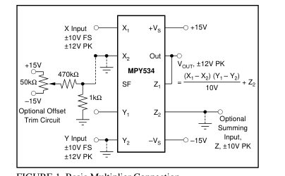
FIGURE 1. Basic Multiplier Connection.
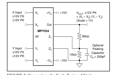
FIGURE 2. Connections for Scale-Factor of Unity.
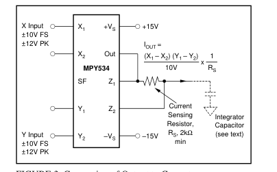
FIGURE 3. Conversion of Output to Current.
DIVIDER CIRCUIT
The MPY534 can be configured as a divider as shown in Figure 4. High impedance differential inputs for the numerator and denominator are achieved at the Z and X inputs, respectively. Feedback is applied to the Y2 input, and Y1 can be summed directly into VOUT. Since the feedback connection is made to a multiplying input, the effective gain of the output op amp varies as a function of the denominator input voltage. Therefore, the bandwidth of the divider function is proportional to the denominator voltage (see Typical Performance Curves).
Page 7
Accuracy of the divider mode typically ranges from 0.75%
to 2.0% for a 10 to 1 denominator range depending on device
grade. Accuracy is primarily limited by input offset voltages
and can be significantly improved by trimming the offset of
the X input. A trim voltage of ±3.5mV applied to the “low
side” X input (X2 for positive input voltages on X1) can
produce similar accuracies over a 100 to 1 denominator
range. To trim, apply a signal which varies from 100mV to
10V at a low frequency (less than 500Hz) to both inputs. An
offset sine wave or ramp is suitable. Since the ratio of the
quantities should be constant, the ideal output would be a
constant 10V. Using AC coupling on an oscilloscope, adjust
the offset control for minimum output voltage variation.
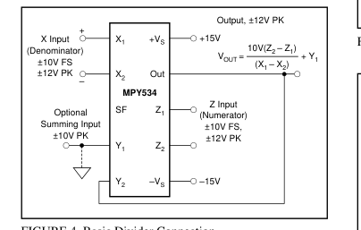
FIGURE 4. Basic Divider Connection.
SQUARE-ROOTER A square-rooter connection is shown in Figure 5. Input
voltage is limited to one polarity (positive for the connection
shown). The diode prevents circuit latch-up should the input
go negative. The circuit can be configured for negative input
and positive output by reversing the polarity of both the X
and Y inputs. The output polarity can be reversed by revers-
ing the diode and X input polarity. A load resistance of
approximately 10kΩ must be provided. Trimming for im-
proved accuracy would be accomplished at the Z input.
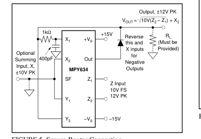
FIGURE 5. Square-Rooter Connection.
APPLICATIONS
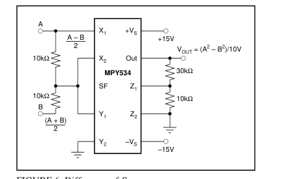
FIGURE 6. Difference-of-Squares.
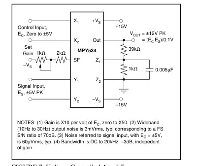
FIGURE 7. Voltage-Controlled Amplifier.
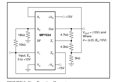
FIGURE 8. Sine-Function Generator.
Page 8
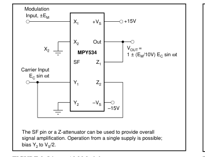
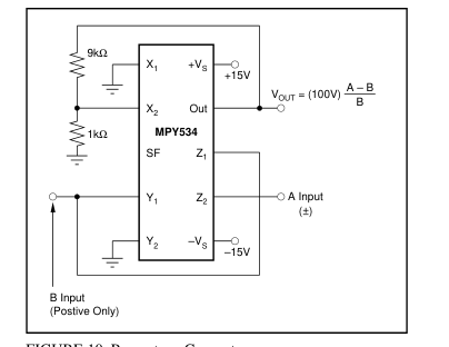
FIGURE 9. Linear AM Modulator.
FIGURE 10. Percentage Computer.
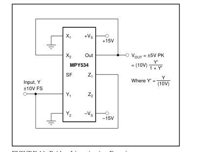
FIGURE 11. Bridge-Linearization Function.
The information provided herein is believed to be reliable; however, BURR-BROWN assumes no responsibility for inaccuracies or omissions. BURR-BROWN assumes no responsibility for the use of this information, and all use of such information shall be entirely at the user’s own risk. Prices and specifications are subject to change without notice. No patent rights or licenses to any of the circuits described herein are implied or granted to any third party. BURR-BROWN does not authorize or warrant any BURR-BROWN product for use in life support devices and/or systems.
Page 9
IMPORTANT NOTICE
Texas Instruments and its subsidiaries (TI) reserve the right to make changes to their products or to discontinue any product or service without notice, and advise customers to obtain the latest version of relevant information to verify, before placing orders, that information being relied on is current and complete. All products are sold subject to the terms and conditions of sale supplied at the time of order acknowledgment, including those pertaining to warranty, patent infringement, and limitation of liability.
TI warrants performance of its semiconductor products to the specifications applicable at the time of sale in accordance with TI’s standard warranty. Testing and other quality control techniques are utilized to the extent TI deems necessary to support this warranty. Specific testing of all parameters of each device is not necessarily performed, except those mandated by government requirements.
Customers are responsible for their applications using TI components.
In order to minimize risks associated with the customer’s applications, adequate design and operating safeguards must be provided by the customer to minimize inherent or procedural hazards.
TI assumes no liability for applications assistance or customer product design. TI does not warrant or represent that any license, either express or implied, is granted under any patent right, copyright, mask work right, or other intellectual property right of TI covering or relating to any combination, machine, or process in which such semiconductor products or services might be or are used. TI’s publication of information regarding any third party’s products or services does not constitute TI’s approval, warranty or endorsement thereof.
Copyright 2000, Texas Instruments Incorporated