
 Download PDF
DDC101 BURR-BROWN
Document overview
- PDF pages: 27
Technical content
Page 1
20-BIT ANALOG-TO-DIGITAL CONVERTER
FEATURES
G MONOLITHIC CHARGE INPUT ADC G DIGITAL FILTER NOISE REDUCTION: 0.9ppm, rms G DIGITAL ERROR CORRECTION: CDS G CONVERSION RATE: Up to 15kHz G USER FRIENDLY EVALUATION FIXTURE
DESCRIPTION
The DDC101 is a precision, wide dynamic range, charge digitizing A/D converter with 20-bit resolution. Low level current output devices, such as photosensors, can be directly connected to its input. The most stringent accuracy requirements of many unipolar output sensor applications occur at low signal levels. To meet this requirement, Burr-Brown developed the adaptive delta modulation architecture of the DDC101 to provide linearly improving noise and linearity errors as the input signal level decreases. The DDC101 combines the functions of current-to-voltage conversion, integration, input programmable gain amplification, A/D conversion, and digital
filtering to produce precision, wide dynamic range re- sults. The input signal can be a low level current connected directly into the unit or a voltage connected through a user selected resistor. Although the DDC101 is optimized for unipolar signals, it can also accurately digitize bipolar input signals. The patented delta modula-
+VS Test In
Test Current Reset
CDAC CINT
18 Bits DAC
Analog
Digital Integration,
Input
Tracking and Control Logic
Ground
Comparator
VREF Setup
APPLICATIONS
G DIRECT PHOTOSENSOR DIGITIZATION G PRECISION INSTRUMENTATION G INFRARED PYROMETRY G PRECISION PROCESS CONTROL G CT SCANNER DAS G CHEMICAL ANALYZERS
tion topology combines charge integration and digitization functions. Oversampling and digital filtering reduce system noise dramatically. Correlated Double Sampling (CDS) captures and eliminates steady state and conversion cycle dependent offset and switching errors that are not eliminated with conventional analog circuits. The DDC101 block diagram is shown below. During conversion, the input signal is collected on the internal integration capacitance for a user determined integration period. A high precision, autozeroed comparator samples the analog input node. Tracking logic updates the internal high resolution D/A converter at a 2MHz rate to maintain
the analog input at virtual ground. A user programmable digital filter oversamples the tracking logic’s output. The digital filter passes a low noise, high resolution digital output to the serial I/O register. The serial outputs of multiple DDC101 units can be easily connected together in series or parallel if desired to minimize interconnections.
DDC101 Integrated Circuit
20 Bits Digital Filter and
Serial In Serial I/O
Error Correction
Serial Out Register
Oversampled Digital Out
International Airport Industrial Park • Mailing Address: PO Box 11400, Tucson, AZ 85734 • Street Address: 6730 S. Tucson Blvd., Tucson, AZ 85706 • Tel: (520) 746-1111 • Twx: 910-952-1111 Internet: http://www.burr-brown.com/ • FAXLine: (800) 548-6133 (US/Canada Only) • Cable: BBRCORP • Telex: 066-6491 • FAX: (520) 889-1510 • Immediate Product Info: (800) 548-6132
©1993 Burr-Brown Corporation
PDS-1211E
Printed in U.S.A. March, 1998
Page 2
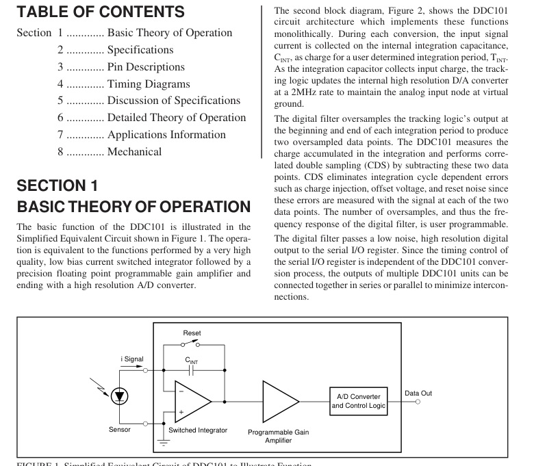
FIGURE 1. Simplified Equivalent Circuit of DDC101 to Illustrate Function.
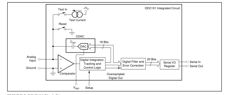
FIGURE 2. DDC101 Block Diagram.
Page 3
An internal test current source is provided for basic func-
tionality testing and diagnostics. This approximately 100nA
current source is pin activated and sums with the external
input current. Figure 3 shows a more detailed circuit configuration of the
DDC101. The single integration capacitor, CINT, and the
D/A converter have been replaced with a high resolution
Capacitor Digital-to-Analog Converter (CDAC). By switch-
ing between ground and VREF the binary weighted capacitor
array of the CDAC accumulates the input signal’s charge to
keep the comparator input at virtual ground.
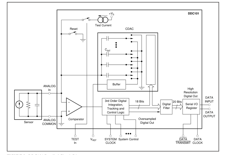
FIGURE 3. DDC101 Detailed Circuit Diagram.
The information provided herein is believed to be reliable; however, BURR-BROWN assumes no responsibility for inaccuracies or omissions. BURR-BROWN assumes no responsibility for the use of this information, and all use of such information shall be entirely at the user’s own risk. Prices and specifications are subject to change without notice. No patent rights or licenses to any of the circuits described herein are implied or granted to any third party. BURR-BROWN does not authorize or warrant any BURR-BROWN product for use in life support devices and/or systems.
Page 4
SECTION 2
SPECIFICATIONS
ELECTRICAL
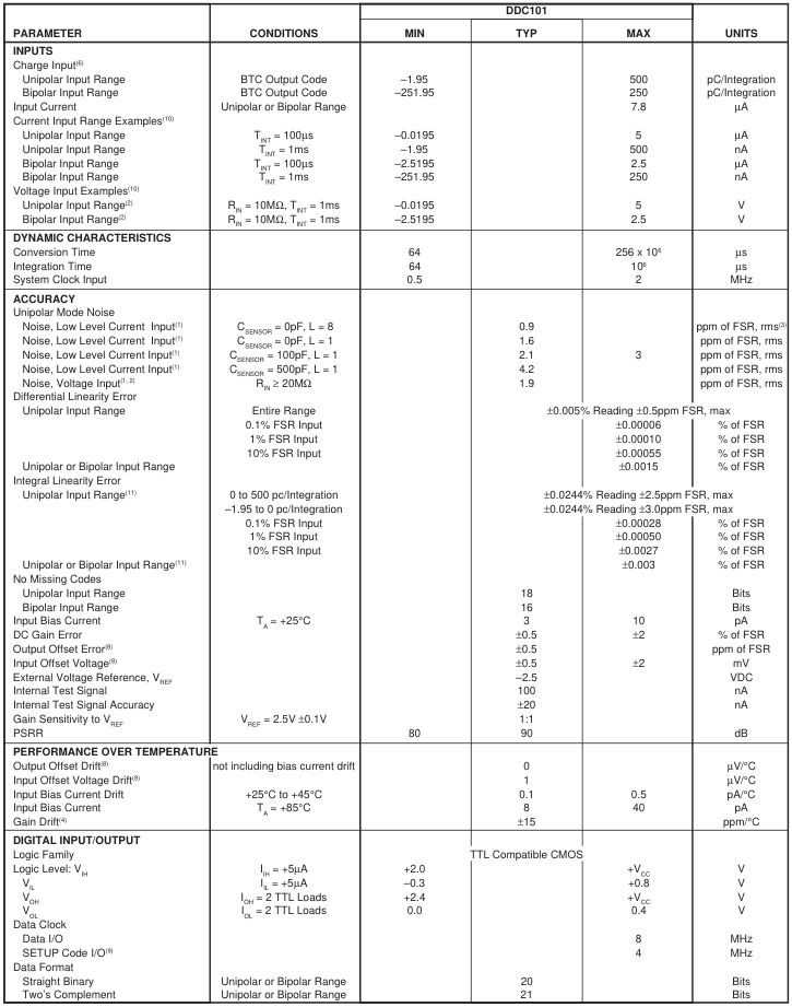
All specifications with unipolar current input range, TINT = 1ms, correlated double sampling enabled, System Clock = 2MHz, VREF = –2.5V, TA = +25°C and VS = ±5VDC, unless otherwise noted.
Page 5
SPECIFICATIONS (CONT)
ELECTRICAL
All specifications with unipolar current input range, TINT = 1ms, correlated double sampling enabled, System Clock = 2MHz, VREF = –2.5V, TA = +25°C and VS = ±5VDC, unless otherwise noted.
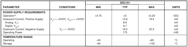
NOTES: (1) Input = low level (less than 1% of Full Scale); Full Scale IIN = 500nA; TINT = 1ms; Unipolar Input Range; Acquisition Time = 16 clock cycles, Oversampling = 128. (2) Voltage input is converted through user provided input resistor, RIN. (3) FSR is Full Scale Range. (4) Gain Drift does not include the drift of the external reference. (5) VDD+ must be less than or equal to VS+. See Section 7 for recommended connections. (6) Straight Binary output code has slightly different Charge Range. See Section 6. (8) Input offset voltage is nulled by autozero circuitry and causes no output error. See Section 6 (Internal Error Correction). (9) This is
the maximum clock frequency at which SETUP codes can be written to and read from the DDC101. (10) For other input current and voltage configurations, see Discussion of Specifications and Detailed Theory of Operation sections. (11) A best-fit straight line method is used to determine linearity. Two different best-fit straight lines are used for the two unipolar integral linearity specifications. Acquisition Time = 16 clock cycles, Oversampling = 128.
PACKAGE/ORDERING INFORMATION
| PRODUCT | PACKAGE | PACKAGE DRAWING NUMBER(1) | THERMAL RESISTANCE (θ ) (°C/W) JA |
| DDC101U | 24-Lead SOIC | 239 | 100 |
NOTE: (1) For detailed drawing and dimension table, please see end of data sheet, or Appendix C of Burr-Brown IC Data Book.
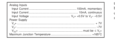
ABSOLUTE MAXIMUM RATINGS
ELECTROSTATIC
DISCHARGE SENSITIVITY
This integrated circuit can be damaged by ESD. Burr-Brown
recommends that all integrated circuits be handled with ap-
propriate precautions. Failure to observe proper handling and
installation procedures can cause damage. ESD damage can range from subtle performance degradation
to complete device failure. Precision integrated circuits may
be more susceptible to damage because very small parametric
changes could cause the device not to meet published
specifications.
The information provided herein is believed to be reliable; however, BURR-BROWN assumes no responsibility for inaccuracies or omissions. BURR-BROWN assumes no responsibility for the use of this information, and all use of such information shall be entirely at the user’s own risk. Prices and specifications are subject to change without notice. No patent rights or licenses to any of the circuits described herein are implied or granted to any third party. BURR-BROWN does not authorize or warrant any BURR-BROWN product for use in life support devices and/or systems.
Page 6
PIN CONFIGURATION
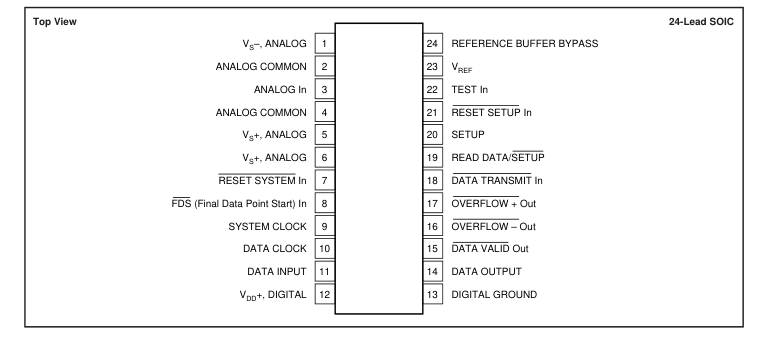
SECTION 3
PIN DESCRIPTIONS
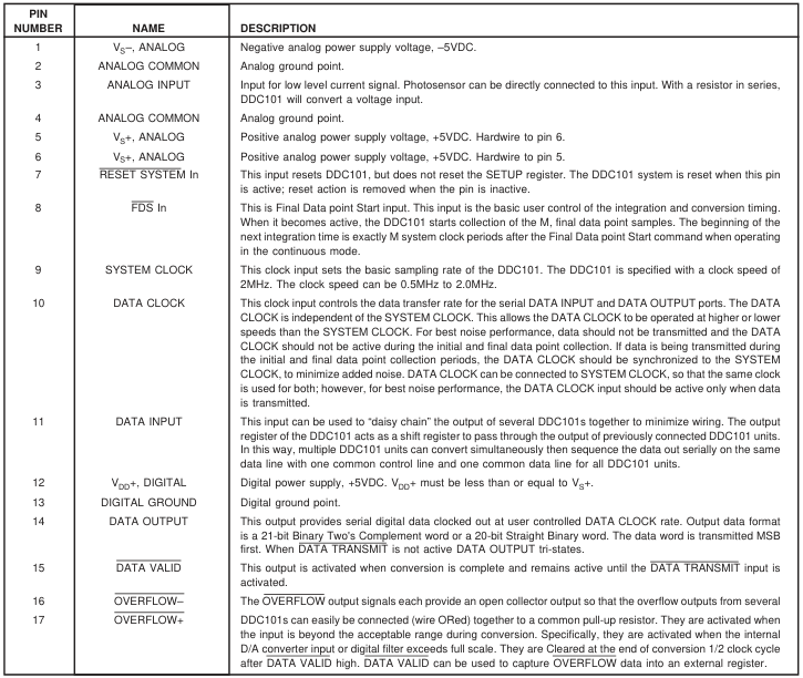
Page 7
PIN DESCRIPTIONS (CONT)
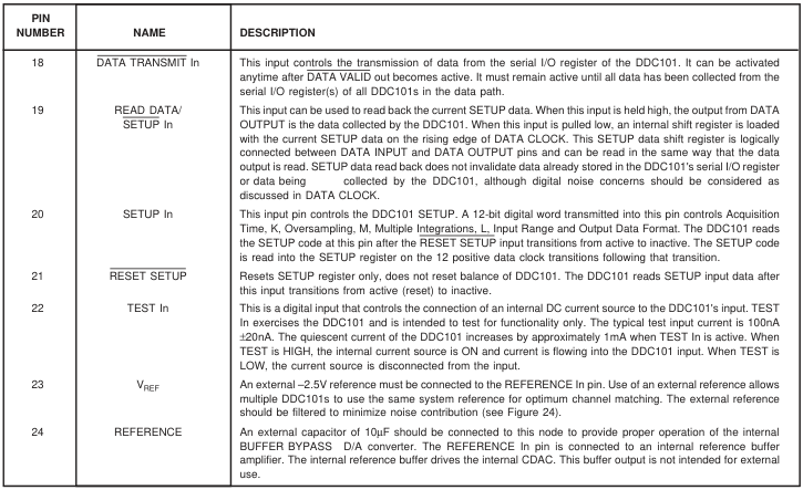
SECTION 4
TIMING CHARACTERISTICS
All specifications with Unipolar input range, TINT = 1ms, Current Input, Correlated Double Sampling enabled, Sys Clock = 2MHz, VREF = –2.5V, TA = +25°C and VS = ±5VDC, unless otherwise noted.
| SYMBOL | DESCRIPTION | MIN | TYP | MAX | UNITS |
|---|---|---|---|---|---|
| t1 t 2 t3 t 4 t5 t 6 t7 t 8 t9 t 10 t11 t 12 t 13 t14 t15 t 16 t17 | FDS Setup FDS width, Continuous Conversion FDS width, Asynchronous Conversion FDS HIGH to start of next integration, Asynchronous Conversion Setup time for RESET SETUP HIGH to DATA CLOCK HIGH Setup time for Setup Codes data valid before rising edge of DATA Clock Hold time for Setup Codes data valid after rising edge of DATA Clock Propagation delay from rising edge of SYSTEM CLOCK to DATA VALID LOW Propagation delay from DATA TRANSMIT LOW to DATA VALID HIGH Setup time for DATA CLOCK LOW to DATA TRANSMIT LOW Propagation delay from DATA TRANSMIT LOW to valid data out Hold time that Data output is valid after falling edge of DATA CLOCK Propagation delay from DATA TRANSMIT HIGH to Data Output tri-stated Propagation delay from falling edge of SYSTEM CLOCK to OVERFLOW+ and OVERFLOW–cleared SYSTEM CLOCK pulse width HIGH SYSTEM CLOCK pulse width LOW DATA VALID LOW to DATA TRANSMIT LOW, Single DDC101 | 30 50 M Clocks+t1 60 30 30 30 10 25 240 240 30 | (M– 50 50 35 30 ( | 1) Clocks+t+1 1 40 LxN–21) Clock | ns 00ns ns ns ns ns ns ns ns ns ns ns ns ns ns ns ns s ns |
Page 8
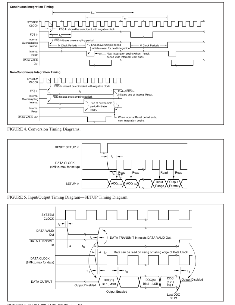
FIGURE 6. DATA TRANSMIT Timing Diagram.
Page 9
TIMING DIAGRAMS (CONT)
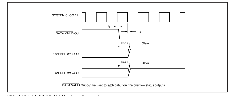
FIGURE 7. OVERFLOW Out Monitoring Timing Diagram.
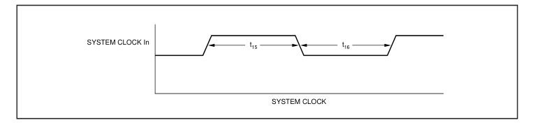
FIGURE 8. System Clock Timing.
Page 10
TYPICAL PERFORMANCE CURVES
ELECTRICAL
System Clock = 2MHz, VS = ±5VDC, VREF = –2.5V, L = 1 Integration/Conversion, and TA = +25°C, unless otherwise noted.
SINAD AT 10kHz CONVERSION, UNIPOLAR INPUT
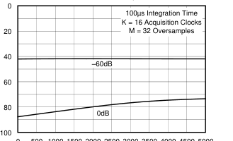
0 500 1000 1500 2000 2500 3000 3500 4000 4500 5000
Input Frequency (Hz)
NOISE vs INPUT LEVEL (UNIPOLAR) WITH CDS
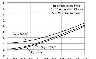
0 0.1 0.2 0.3 0.4 0.5 0.6 0.7 0.8 0.9 1.0
Input Level of FS
NOISE vs RESISTOR VALUE
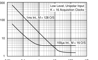
0.01 0.1 1 10 100 1G
RIN (MΩ)
SINAD AT 1kHz CONVERSION, UNIPOLAR INPUT
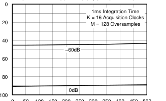
0 50 100 150 200 250 300 350 400 450 500
Input Frequency (Hz)
NOISE vs INPUT LEVEL (UNIPOLAR) WITHOUT CDS
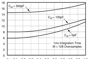
0 0.1 0.2 0.3 0.4 0.5 0.6 0.7 0.8 0.9 1.0
Input Level of FS
CHARGE INJECTION vs INPUT CAPACITANCE
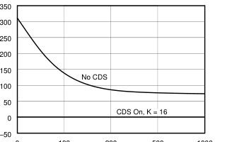
0 100 200 500 1000
CIN (pF)
Page 11
TYPICAL PERFORMANCE CURVES (CONT)
ELECTRICAL
System Clock = 2MHz, VS = ±5VDC, VREF = –2.5V, L = 1 Integration/Conversion, and TA = +25°C, unless otherwise noted.
NOISE vs INPUT CAPACITANCE, UNIPOLAR INPUT
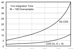
0 100 200 500 1000 2000
CIN (pF)
CHANGE IN IB vs TEMPERATURE
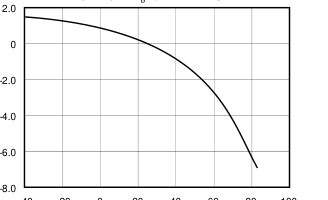
–40 –20 0 20 40 60 80 100
Temperature (°C)
NOISE vs INTEGRATION TIME, UNIPOLAR INPUT
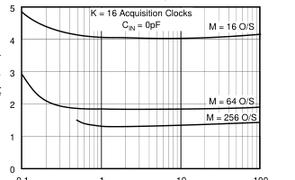
0.1
1
10
100
Integration Time (ms)
NOISE vs OVERSAMPLING, UNIPOLAR INPUT
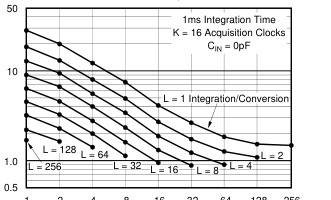
1 2 4 8 16 32 64 128 256
M Oversamples
NOISE vs TEMPERATURE, UNIPOLAR INPUT
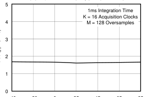
–40 –20 0 25 45 65 85
Temperature (°C)
INPUT OFFSET VOLTAGE vs INPUT CAPACITANCE
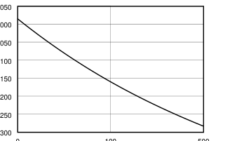
0.050
0.000
–0.050
0.100
–0.150
–0.200
–0.250
–0.300 0
100
500
CIN (pF)
Page 12
TYPICAL PERFORMANCE CURVES (CONT)
ELECTRICAL
System Clock = 2MHz, VS = ±5VDC, VREF = –2.5V, L = 1 Integration/Conversion, and TA = +25°C, unless otherwise noted.
NEGATIVE PSRR vs FREQUENCY
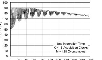
0 20 40 60 80 100 120 140 160 180 200
Frequency (kHz)
NEGATIVE PSRR vs FREQUENCY
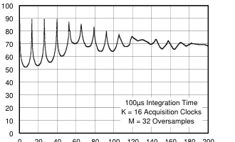
0 20 40 60 80 100 120 140 160 180 200
Frequency (kHz)
POSITIVE PSRR vs FREQUENCY
0 20 40
60 80 100 120 140 160 180 200 Frequency (kHz)
POSITIVE PSRR vs FREQUENCY
0 20 40
60 80 100 120 140 160 180 200 Frequency (kHz)
Page 13
SECTION 5
DISCUSSION OF
SPECIFICATIONS
INPUT
The DDC101 is a charge digitizing A/D converter. Low level current output sources, such as a photosensors, can be directly connected to its input. The input signal can also be a voltage connected through a user selected resistor.
CHARGE INPUT
The maximum charge that can be captured in one integration by the DDC101 is 500pC. In the unipolar input range mode, the maximum positive charge that can be collected in one integration is 500pC. The DDC101 has a small negative range in the unipolar mode of –1.95pC. This small negative underrange is included to allow for a small amount of leakage current from the user’s PC board and sensor. In the bipolar input range, the maximum positive charge that can be collected is +250pC. The maximum negative charge that can be collected is –251.95pC. In addition to the normal mode of one integration per conversion, DDC101 can be configured by the user for 1 to 256 integrations per conversion. When the multiple integra-
tions per conversion mode is chosen, the DDC101 DSP circuitry internally averages multiple integration cycles to provide one conversion result. This result has lower noise because it is the average of multiple integrations. In this mode, the maximum total charge that can be captured by the DDC101 in 256 integrations is 128,000pC.
TEST CURRENT INPUT
An internal DC test current can be connected under user control to the DDC101’s input. The test current is nominally 100nA and will be summed with any applied external input signal. It is derived by a resistive network from the positive power supply. The test current is intended to test for functionality only. The TEST In pin of the DDC101 controls the current. When TEST is HIGH, the internal current source is ON and current is flowing into the DDC101 input. When TEST is LOW, the current source is disconnected from the input. With TEST active, positive power supply current increases by approximately 1mA.
FULL SCALE RANGE
The full scale range (FSR), which is referenced in the specification table, is the difference between the positive full scale charge and the negative full scale charge for the DDC101 in one integration cycle. Specifications such as noise and linearity, which are specified in percent or ppm of FSR, are referring to a value of 500pC for both unipolar and bipolar input ranges. The full scale input current for a given integration time will result in a full scale input charge. As an example for unipolar
input range, an input current of 0.5µA integrated for 1ms will result in the full scale charge of 500pC. For voltage inputs, the input resistor is chosen to achieve the proper full scale input current. As an example, for a 5V full scale input, a 10MΩ input resistor is selected to achieve a full scale input current of 0.5µA (1ms integration time). Noise of 1.6ppm of FSR is equal to 1.6ppm x 500pC = 0.8fC or 1.6ppm x 0.5µA = 0.8pA or 1.6ppm x 5V = 8µV. Thus, in this instance, noise is 1.6pA or 8µV. For the unipolar input range, the following table shows the full scale input current required for different integration times to collect 500pC of charge and the equivalent current
values for 2 and 5ppm of FSR.
| T INT | I FS | 2ppm | 5ppm |
| 50ms 5ms 1ms 500µs 100µs | 10nA 100nA 500nA 1µA 5µA | 0.02pA 0.2pA 1pA 2pA 10pA | 0.5pA 1pA 2.5pA 5pA 25pA |
TABLE I. Integration Time (TINT) and Full Scale Current (IFS) for Full Scale 500pC Integration.
CURRENT INPUT
The maximum average input current that can be captured by the DDC101 is ±7.8µA. This current will result in an integration time of 64µs for unipolar input range and 32µs for bipolar input range. For longer integration times, the average input current must be less. The maximum input current is limited by the slew and update rate of the internal tracking logic and CDAC. The largest input current that the DDC101 can accurately track is 7.8µA. Input currents larger than 7.8µA and high speed current input pulses can be accurately captured and digitized by the DDC101 with an external input or sensor capacitance on the DDC101 input. The average current during a com-
plete integration cycle cannot exceed 7.8µA. Likewise, the total charge input must not exceed 500pC unipolar, 250pC bipolar during the integration time. An external user provided input capacitance, CS, as shown in Figure 9a, will capture the input signal charge if the input current limit is temporarily exceeded during the integration cycle. The DDC101 will then transfer the charge completely to CINT based upon conservation of charge. An additional
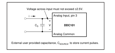
FIGURE 9a. Current Pulse Input Capture.
Page 14
constraint is, the voltage that appears at the DDC101 input, must not exceed 2.5V. If this voltage is exceeded, charge may be lost and the integration result may be invalid. The input voltage can be calculated:
dv i(t) = CS dt or V = 1 i(t)dt ∫ CS therefore, V = i t . CS
As an example, with a user supplied input capacitance of 100pF, a current pulse of 100µA for 2µs could be stored without exceeding 2.5V applied to the input:
2µs ( ) • V = 100µA
= 2V. 100pF
The current pulse must occur completely during part of one DDC101 integration time, and the DDC101 must still have time to discharge the input capacitance to ground at a maximum rate of 7.8µA before the DDC101 is triggered (through the FDS input) to end the integration. In addition, the total charge integrated must be 500pC or less for the unipolar range. A current pulse of 100µA for 2µs creates 200pC of charge.
VOLTAGE INPUT SPECIFICATIONS
The DDC101 is a charge digitizing device. With a user provided input resistor, the DDC101 can digitize voltage inputs. All of the general charge/current input specifications apply to the voltage input situation. The specification table shows the typical noise of the DDC101 including the effects of a 20MΩ input resistor, RIN. The input of the DDC101 is a virtual ground. A voltage input causes a current, i, to flow into the input through RIN as shown in Figure 9b. The maximum input current is determined by the integration time selected. Table II shows the
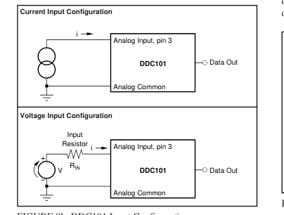
FIGURE 9b. DDC101 Input Configurations.
maximum input voltage based upon several selections of input current and input resistor for unipolar input range. The accuracy of the input resistor will add directly to the DC Gain Error of the DDC101; the drift of the input resistor will add directly to the Gain Drift of the DDC101. Note that the DDC101 output noise decreases as RIN in- creases. This is because the DDC101 noise gain decreases and the input resistance current noise decreases as RIN increases. This effect is shown in the “Noise vs Resistor Value” typical performance curve.
| INTEGRATION TIME | INPUT RESISTOR, R IN | ||
| 1ms | 500µs | 100µs | |
| Full Scale Input Current | 0.5µA | 1µA | 5µA |
| Full Scale Voltage 50mV 500mV 5V 50V | 100kΩ 1MΩ 10MΩ 100MΩ | 50kΩ 500kΩ 5MΩ 50MΩ | 10kΩ 100kΩ 1MΩ 10MΩ |
TABLE II. Example of Input Resistor Values Unipolar Input Range.
UNIPOLAR LINEARITY ERRORS
Due to innovative design techniques, the absolute level of linearity error of the DDC101 improves as the input signal level decreases when used in the unipolar input mode. Therefore, in unipolar input mode, the integral linearity of the DDC101 is specified as a small base error plus a percentage of reading error or as a percentage of full scale range. A best-fit straight line method is used to determine integral linearity. Two different best-fit straight lines are used for the two unipolar integral linearity specifications. For bipolar input mode, linearity is specified only as a percentage of full scale range. To illustrate the improvement in unipolar mode linearity
error, Figure 10 shows the maximum unipolar integral linearity error (ILE) of the DDC101 as a function of the input signal level. The maximum integral linearity error is ±0.0244% of reading ±2.5ppm of FSR (ILE max for unipolar input of –1.95 to 0 pc is ±0.0244% of reading ±3.0ppm of FSR). Thus, the maximum ILE for an input level of 1% of FSR is 0.0005%FSR.
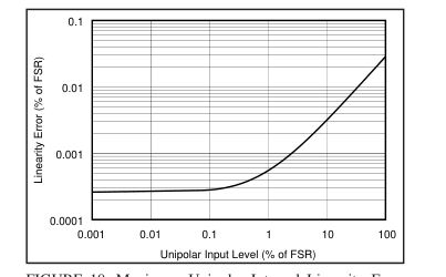
FIGURE 10. Maximum Unipolar Integral Linearity Error
Relative to Full-Scale, Converted From % of Reading Specification.
Page 15
NOISE
The noise of the DDC101 improves as the input signal level decreases, thus very low level signals can be resolved. Noise is shown in the specification table for low level inputs. For unipolar input range, the DDC101 noise at low level inputs is dominated by comparator noise gained to the output; at full scale inputs, the noise is dominated by D/A converter noise. The noise at low low level inputs is a function of input capacitance; the noise at full scale is relatively independent of input capacitance. For bipolar input operation, the noise is dominated by D/A converter noise and is higher than the full scale unipolar noise.
BIPOLAR INPUT ACCURACY
Linearity—As a bipolar input device, the linearity of the DDC101 is specified as a percentage of full scale range that does not improve with lower input signal levels. Performance is generally limited by the linearity of the unit when operated in the bipolar input mode. Noise—In general, noise is not as important as linearity when determining total error. The output noise of the DDC101 in the bipolar mode peaks at midscale (zero input signal level). Output noise is lower for inputs above and below zero.
RESET CHARGE ERROR
The reset charge error (typically less than 250fC) is an offset error that could result from offset voltage, charge injection and kT/C errors. The DDC101 eliminates the effects of reset charge errors with correlated double sampling.
DC BIAS VOLTAGE
The DDC101 generates a small bias voltage (typically 500µV) at the input. This voltage is impressed on any sensor that is connected to the input. The DC bias voltage is the actual virtual ground voltage of the DDC101. The DDC101 input comparator circuitry includes an autozero circuit which eliminates this offset internally so that it does not produce an output error.
GAIN SENSITIVITY TO VREF
The DDC101 gain is dependent upon the external reference voltage, VREF. A change in the value of VREF will be seen as a directly proportional change in the gain of the DDC101.
FREQUENCY RESPONSE
The DDC101 is a sampling system whose transfer function has three separate frequency components. These components are multiplied together to make the total frequency characteristic of the DDC101. The three components are: 1. Basic Integration This is the characteristic sin(x)/x response of the basic integration function. This response is controlled by the integration time of the DDC101.
- Oversampling This is the low pass filter characteristic of the digital filter’s oversampling. This response reduces the broadband noise in the input signal and the DDC101. Broadband noise decreases as the number of oversamples increases. 3. Multiple Integrations This is the low pass filter characteristic that results when the digital filter is used to average multiple integrations. This will determine the primary response of the DDC101 if two or more integrations are internally averaged. See Section 6 for more details.
SECTION 6
DETAILED THEORY
OF OPERATION
INTEGRATION CYCLE
An integration cycle, as illustrated in Figure 11, includes the Acquisition Time, Initial Data Point Sampling, Tracking Interval, and Final Data Point Sampling. The Acquisition Time is K clock periods. The first clock cycle of the Acquisition Time is used to reset the integrating capacitor, CINT, to zero from the previous integration. The balance of the Acquisition Time insures that the DDC101 system is accurately tracking the input signal prior to initial data point acquisition. Close-ups of the Reset and Acquisition time are shown in Figures 12 and 13. The Initial Data Point is then sampled M times. The Integration cycle time consists primarily of the Tracking Interval
during which time the DDC101 “tracks” the integration of the input signal. The Tracking Interval is followed by the measurement of the Final Data Point with the same user selected number of samples, M. M and K are user selectable. The entire integration cycle consists of N clock periods as controlled by the user. The DDC101 operates in continuous and non-continuous integration modes. In the continuous mode, one integration follows another with no delay from the end of one integration to the beginning of the next conversion. In the noncontinuous mode, each new integration is started separately under user control. The Final Data point Start (FDS) input is the primary user
control of the integration cycle. The FDS input controls the end of one integration cycle and the start of the next integration cycle in both the continuous and non-continuous integration modes. Measurement of the M final data point samples begins when the FDS input is activated.
CONTINUOUS INTEGRATION MODE
In the continuous integration mode, the “Final Data Point Start” command (using the FDS pin) initiates the measurement of the M final data point samples. The next integration cycle begins immediately after the final data point sampling
Page 16
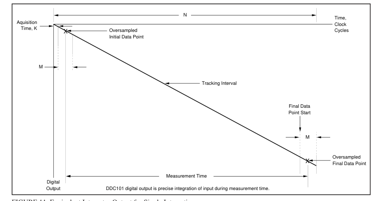
FIGURE 11. Equivalent Integrator Output for Single Integration.
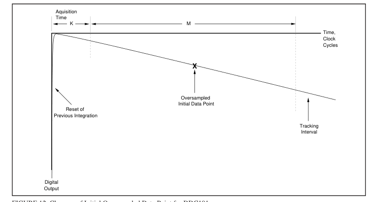
FIGURE 12. Close-up of Initial Oversampled Data Point for DDC101.
has been completed; this occurs M clock periods after the FDS transition to “ON”. Acquisition, Initial Data Point and Tracking for the next integration follow automatically. The DDC101 continues in the Tracking mode until the next FDS command initiates the measurement of the M final data point samples. An FDS command is needed for each integration cycle. In the continuous integration mode, the FDS pulse width must be less than M clock periods. If the FDS pulse
is held low past this time of M clock periods, the DDC101 will reset as for non-continuous mode (see also Figure 4). In the continuous mode of operation, the tracking logic of the DDC101 “remembers” the integration rate of the previous integration and begins the next integration at the rate of the previous integration. This allows faster acquisition of the signal for the next integration.
Page 17
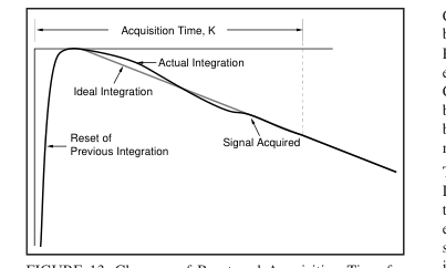
FIGURE 13. Close-up of Reset and Acquisition Time for
DDC101.
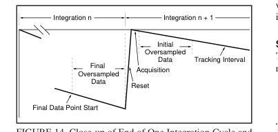
FIGURE 14. Close-up of End of One Integration Cycle and
Beginning of Next.
NON-CONTINUOUS INTEGRATION MODE
For the non-continuous integration mode, FDS controls the start of the M final data point samples and the end of integration as discussed above. In this mode, however, FDS is also used to control the start of a new integration cycle asynchronously with the end of the previous integration. When FDS transitions to “ON”, the collection of the M final data point samples begins. At the end of each integration, the DDC101 automatically resets the integration capacitance. If FDS remains “ON” past the end of integration, the DDC101 will stay in the integration reset state until FDS transitions to “OFF”. Holding FDS “ON” past the end of integration will also reset the DDC101’s tracking logic to zero integration
rate. In non-continuous integration mode, the initial data point measurement may be less accurate since the DDC101’s internal tracking logic is reset at the beginning of the integration and tracking may not be accurate for the initial data point measurement. In this situation, Correlated Double Sampling (CDS) operation may not be advantageous.
INTERNAL ERROR CORRECTION
The DDC101 uses CDS techniques to gain optimum performance. CDS removes internal DDC101 errors which occur for a given integration cycle such as, charge injection, kT/C, and DDC101 offset errors. Correlated Double Sampling is user selectable. It is recommended for most continuous measurement applications.
Correlated Double Sampling is implemented in the DDC101 by subtracting the Initial Data Point from the Final Data Point. Thus, the error correction is updated automatically for each integration. When operating in the unipolar input range, CDS functions with either output data format—straight binary or binary two’s complement. When operating in the bipolar input range, CDS functions with binary two’s complement output data format only. The errors that CDS removes are charge injection, kT/C and DDC101 input voltage offset. These errors are very difficult to eliminate in equivalent analog circuits. Charge injection errors result from charge that is transferred through the reset
switch into the integration capacitor. kT/C errors are switching errors due to the noise of the resistance of the reset switch. DDC101 voltage offset errors are due to input offset of the input comparator. Both initial offset and offset drift with time and temperature are corrected since the correction is performed each integration cycle.
SINGLE CYCLE INTEGRATION
The DDC101 acquires charge (q) by integrating input current (i) for a specific time (T). That is,
T ∫ dt q = i O
The DDC101 acquires up to 500pC of full scale charge per integration cycle in the unipolar input range, and approximately ±250pC of full scale charge in the bipolar input range. Therefore, for the DDC101, maximum values can be calculated. Unipolar Input Range Bipolar Input Range 500pC = IFS x TINT
±250pC = ±IFS x TINT
Where IFS is the full scale input current and TINT is the integration time of the DDC101. Examples of IFS and TINT that equal 500pC and ±250pC are shown in the following tables. The maximum average input current that the DDC101 can integrate is 7.8µA. This results in a minimum integration time of 64µs for unipolar inputs and 32µs for bipolar inputs. Further flexibility is possible with multiple integration cycles per conversion as described in the following text.
INPUT RANGE
Unipolar Input Range For the unipolar input range, the range of charge for each integration cycle is from positive full scale of +500pC to a slightly negative charge of –1/256 (approximately –0.4%) of the positive full scale charge. This is +500pC to –1.95pC. The negative charge measurement capability allows for low level PC board parasitic leakages.
Bipolar Input Range For the bipolar input range, the range of charge for each integration cycle is from positive full scale of +250pC to negative full scale of –251.95pC.
Page 18
| I FS | T INT |
| 1nA 10nA 100nA 1µA 5µA 7.8µA | 500ms 50ms 5ms 500µs 100µs 64µs |
TABLE III. Input Current vs Integration Time Examples
for Maximum Charge. Unipolar input range maximum charge = 500pC.
| ±IFS | TINT |
| 1nA 10nA 100nA 1µA 2.5µA 7.8µA | 250ms 25ms 2.5ms 250µs 100µs 32µs |
TABLE IV. Input Current vs Integration Time Examples
for Maximum Charge. Bipolar input range maximum charge = ±250pC.
MULTIPLE INTEGRATIONS
PER CONVERSION CYCLE
If more than 500pC, unipolar (or ±250pC, bipolar) of charge must be integrated in one conversion cycle, the DDC101 can be user programmed for multiple integrations per conversion cycle. This feature can be used to provide for longer conversion periods for a specific input current other than shown in the previous table. The integration cycles forming a conversion cycle may be continuous or non-continuous. The number of integrations per conversion cycle, L, can be 1, 2, 4, 8, 16, 32, 64, 128, or 256. The multiple integrations are automatically averaged in the DDC101 so that one conversion result is output per total conversion cycle. Note that each integration requires individual control by the FDS
signal. For example, if L = 4, then four FDS signals per conversion are required.
FINAL DATA POINT CONFIGURATION LIMITS
In each conversion cycle, the maximum number of final data points which can be collected is 256. This means that at the extremes, the DDC101 can be setup to perform one integration cycle with 256 oversamples, or the DDC101 can be setup to perform 256 integration cycles with one sample per integration cycle. The total number of integrations, L, multiplied by the number of samples per final data point, must be 256 or less. As an example, if 16 integration cycles, L, are used, the number of samples per final data point must be 16 or less. NOTE: When CDS is used, the initial data points impose no additional conversion sampling limitations.
FREQUENCY RESPONSE
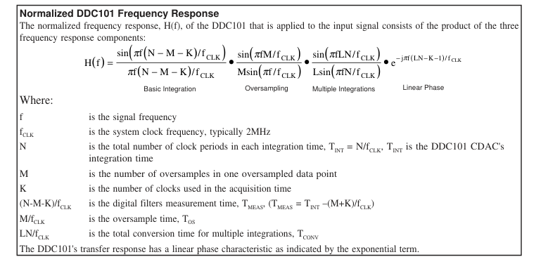
The DDC101 charge digitizing A/D Converter is a sampled system whose frequency response has three separate components. These components are multiplied together to make the total frequency characteristic of the DDC101. The three frequency response components are shown below. Each
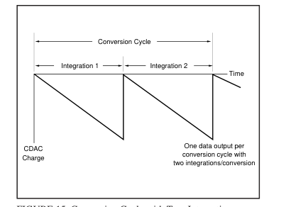
FIGURE 15. Conversion Cycle with Two Integrations.
| INTEGRATIONS PER CONVERSION | I FS | CONVERSION TIME | MAX CHARGE/ CONVERSION |
|---|---|---|---|
| L = 1 L = 2 L = 4 L = 8 L = 16 L = 32 L = 64 L = 128 L = 256 | 10nA 10nA 10nA 10nA 10nA 10nA 10nA 10nA 10nA | 50ms 100ms 200ms 400ms 800ms 1.6s 3.2s 6.4s 12.8s | 500pC 1000pC 2000pC 4000pC 8000pC 16000pC 32000pC 64000pC 128000pC |
TABLE V. Integrations/Conversion vs Conversion Time. Example for multiple integrations with unipolar input range.
individual component has a sinc (sinx/x) frequency response function. 1. Basic Integration This is the characteristic sin(x)/x response of the basic integration function. This response is controlled by the measurement time of the DDC101, TMEAS; see Figure 16. 2. Oversampling This is the low pass filter characteristic of the digital filter’s oversampling. This response reduces the broadband noise in the input signal of the DDC101. Broadband noise decreases as the number of oversamples increases. This response is controlled by the number of oversamples, M; see Figure 17. 3. Multiple Integrations This is the low pass filter characteristic that results when the digital filter is used to average multiple integrations.
This will determine the primary response of the DDC101 if two or more integrations are internally averaged. This response is controlled by the total conversion time of the DDC101; see Figure 18. Input frequencies are multiplied by the DDC101 frequency response. The Nyquist frequency is fCONV/2, where fCONV is the DDC101 conversion rate. The highest frequency that can be reconstructed from the output data is fCONV/2. Input frequencies above Nyquist are multiplied by the DDC101 frequency response and are then aliased into DC to fCONV/2.
Page 19
Basic Integration Frequency Response The sin(x)/x basic integration characteristic is controlled by the digital filter’s measurement time (TMEAS). The measurement frequency, fMEAS is l/TMEAS. The input frequency re- sponse of the DDC101 is down –3dB at fMEAS/2.26 with a null at fMEAS. Subsequent nulls are at harmonics 2fMEAS, 3fMEAS, 4fMEAS, etc. as shown in the frequency response curve below. This characteristic is often used to eliminate known interference by setting fMEAS or a harmonic to exactly the frequency of the interference. Table VI illustrates the frequency characteristics of the DDC101 integration function for various measurement times. As an example, for N =
2272, K = 16, and M = 256: TMEAS = (N-M-K)/fCLK = (2272- 256-16)/2MHz = 1ms and fMEAS = 1kHz. TINT = 2272/2MHz = 1.14ms; fCONV = l/TINT = 880Hz.
| MEASUREMENT TIME | –3dB FREQUENCY | f MEAS |
| 100µs 1ms 10ms 16.66ms 20ms | 4.42kHz 442Hz 44.2Hz 26.5Hz 22.1Hz | 10kHz 1kHz 100Hz 60Hz 50Hz |
TABLE VI. Basic Integration Frequency Response Examples.
Oversampling Frequency Response The M oversamples of the initial and the final data points create an oversampling sin(x)/x type of low pass filter response. The oversampling function reduces broadband noise of the input signal and the DDC101. Broadband noise is reduced approximately in proportion to the square root of the number of oversamples, M. As an example, a conversion with 128 oversamples will have approximately 1/2 the noise of a conversion with 32 oversamples (√32/128 = √1/4 = 1/2) The oversampling low pass filter response creates a null
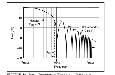
FIGURE 16. Basic Integration Frequency Response.
at fOS = 1/TOS. The oversample time, TOS, is M/fCLK. For M = 256 and fCLK = 2MHz, fOS is approximately 7.8kHz. Subsequent nulls are at harmonics 2fOS, 3fOS, 4fOS, etc. The –3dB point is at fOS/2.26. Table VII illustrates the DDC101 oversampling frequency characteristics with approximate values for fOS and the –3dB frequency. An oversampling frequency response graph is shown below in Figure 17. This figure shows the frequency response for M = 256 oversamples with an fCLK of 2MHz . The slope of the attenuation curve decreases at approximately 20dB/decade.
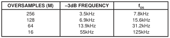
TABLE VII. Oversample Frequency Response Examples.
Page 20
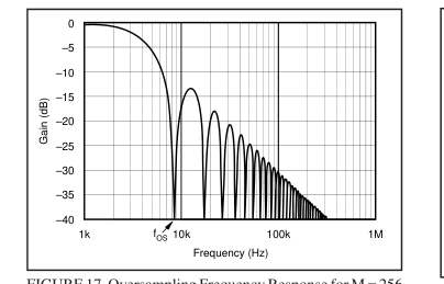
FIGURE 17. Oversampling Frequency Response for M = 256
(fCLK = 2MHz).
Multiple Integration Frequency Response If the DDC101 is operated in the multiple integrations per conversion mode of operation, an additional sin(x)/x type low pass filter is created. The filter creates an initial null frequency at the conversion frequency, fCONV of the DDC101 and at multiples of fCONV. The –3dB point for this filter is also at fCONV/2.26. The conversion time, TCONV, is the sum of the integration times for multiple integrations that are averaged together by the DDC101. TCONV = LN/fCLK. fCONV = l/TCONV. If multiple integrations per conversion are used, this filter will be the dominant low frequency filter of the DDC101. Table VIII shows examples of the conversion time and
frequency for different parameter selections. Figure 18 shows an example of the frequency response due to Multiple Integrations. In the case of Figure 18, the integration time is 500µs (N = 1000 clock periods) and L = 64 integrations per conversion.
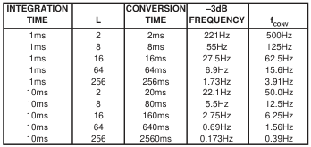
TABLE VIII. Multiple Integration Time Examples.
System Noise implications The noise at the digital output of the DDC101 consists of system noise that is included in the analog input signal and noise from the DDC101. DDC101 Noise—The noise of the DDC101 includes low frequency and broadband noise. The low frequency noise is reduced by the integrating function and the CDS function of the DDC101. This is reflected in the basic integration frequency response and in the multiple integration frequency response. The broadband electronic noise is reduced primarily by the oversampling function of the DDC101
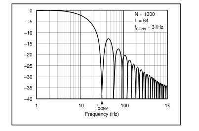
FIGURE 18. A Multiple Integration Frequency Response
Example.
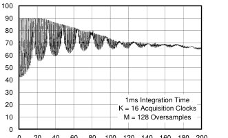
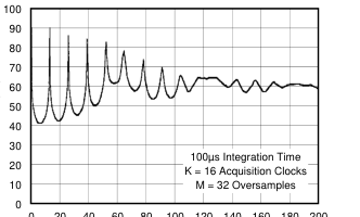
Signal Noise—The noise of the input signal is filtered and reduced in a manner similar to the DDC101 noise reduction through the integrating and oversampling functions of the DDC101. Figures 19 and 20 show the frequency response of the DDC101 for the product of the basic integration and oversampling frequency response for two different values of M. In both examples, the integration time is 1ms, the only difference is in the number of oversamples, M; for Figure 19, M = 256 oversamples was used; for Figure 20, M = 32 oversamples was used. The first null frequency is fMEAS and subsequent nulls are at multiples of fMEAS. The first example with the larger number of oversamples (M = 256) clearly
reduces high frequency noise more than the second example with M = 32. For M = 256, fOS is 7.8kHz, fMEAS is 1.16kHz, and the –3dB frequency is 507Hz. For M = 32, fOS is 62.4kHz, fMEAS is 1.02kHz and the –3dB frequency is 453Hz.
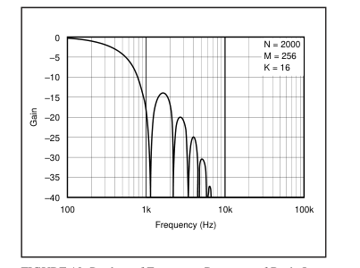
FIGURE 19. Product of Frequency Response of Basic Inte-
gration and Oversampling: 1ms Integration Time, 256 Oversamples.
Page 21
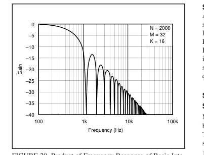
FIGURE 20. Product of Frequency Response of Basic Inte-
gration and Oversampling; 1ms Integration Time, 32 Oversamples.
Figure 21 shows the frequency response of the DDC101 and an ideal integrator with the same integration time. In this comparison, the DDC101 has greater bandwidth to the first null, but it also has greater out of band attenuation which reduces broadband noise significantly. If desired, the frequency response of the ideal integrator can be produced by passing the DDC101 output through an external digital filtering function which has the frequency response from DC to Nyquist of
πfTINT sin(πfTMEAS) • Msin(πf / f CLK )
πfTMEAS
sin(πfTINT )
sin(πfM / f CLK ) .
This has the effect of further attenuating undesired signals (noise) outside the “passband”, further increasing the signalto-noise ratio of the DDC101 and closely emulating the ideal integrator’s signal accumulation characteristics.
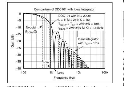
FIGURE 21. Comparison of DDC101 with Ideal Integrator.
SYSTEM SETUP
After power up, the Reset System and FDS signal inputs should be held low (active), while the SETUP register is loaded by the user. After the SETUP register is loaded, the Reset System input should transition to inactive while the FDS input remains active. The FDS should transition to inactive at the start of operation. Thereafter, Reset System should stay inactive and the FDS should be used to control each integration cycle.
SETUP INPUT
Software Control Many of the options of the DDC101 are set through a serial bit stream transmitted by the user into the SETUP Input pin. The 12-bit word transmitted into the SETUP Input is used to set the following four options, in sequence: 1. Acquisition Time Control, K
2 bits
- Oversampling Control Samples/Integration, M
4 bits
- Multiple Integration Control Integrations/Conversion, L
4 bits
- Unipolar or Bipolar Input Range
1 bit
- Output Format
1 bit
Total for SETUP
12 bits
See Figure 5: SETUP Timing Diagram.
Acquisition Time Control, K This signal sets the acquisition time (K clock periods) and controls the use of Correlated Double Sampling. The acquisition time occurs at the start of each new integration. The acquisition time control can be set to four options: “no CDS”, 1, 16 or 32 clock periods. For typical continuous integration applications, K = 16 is recommended. The acquisition time always begins with one clock period for reset. This reset clock period is followed by 0, 15 or 31 clock periods for signal acquisition. Correlated Double Sampling is activated if the initial acquisition time is set to 1, 16 or 32 clock periods. Correlated Double Sampling is disabled and
the Initial Data Point is not acquired if “no CDS” is selected.
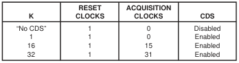
TABLE IX. Acquisition Time Control, K.
When Correlated Double Sampling is activated, the DDC101 acquires the initial data point for error correction as part of each conversion. At the end of the conversion cycle, the initial data point is subtracted from the final data point. The errors that are corrected with CDS are charge injection, kT/C noise, and DDC101 voltage offset. When Correlated Double Sampling is deactivated, the initial data point is not taken.
Page 22
When operating in the unipolar input range, CDS functions with either output data format—straight binary or binary two’s complement. When operating in the bipolar input range, CDS functions correctly only with binary two’s complement output data format.
Oversampling Control Samples/Integration, M This control sets the number of samples, M, used by the DDC101 to oversample the initial and final data points. M can be set for these values: 1, 2, 4, 8, 16, 32, 64, 128, 256. Broadband noise in the conversion is reduced roughly in proportion to the square root of M. Therefore, a conversion with 128 oversamples will have 1/2 the broadband noise of a conversion with 32 oversamples. See the previous frequency response discussion.
Multiple Integration Control, L This control sets the number of integrations per conversion cycle, L. It is used to reduce the data rate, increase the magnitude of the input signal range, and/or reduce the noise. The product of L and M must be 256 or less.
Output Format Two output formats are available for either the unipolar or bipolar input ranges: Binary Two’s Complement (BTC) and Straight Binary.
UNIPOLAR INPUT RANGE
For Binary Two’s Complement, output data format, the output word is a 21-bit Two’s Complement word. The first bit is the sign bit followed by the Most Significant Bit (MSB), etc. The output range is +100%FS to –0.4%FS, where FS is 500pC.
| CODE | INPUT SIGNAL | |
| 0 1111 1111 1111 1111 1111 0 1111 1111 1111 1111 1110 0 0000 0000 0000 0000 0001 0 0000 0000 0000 0000 0000 1 1111 1111 1111 1111 1111 1 1111 1111 0000 0000 0000 | +100%FS +100%FS –1LSB +1SLB Zero –1LSB –0.4%FS | +500pC 0pC –1.95pC |
TABLE X. BTC Code Table—Unipolar Input Range.
For Straight Binary output data format, the output is a 20-bit straight binary word. The first bit is the Most Significant Bit (MSB), etc. The output range is +99.6%FS to –0.4%FS in which +99.6%FS represents positive full scale and –0.4%FS represents the minimum input.
| CODE | INPUT SIGNAL | |
| 1111 1111 1111 1111 1111 1111 1111 1111 1111 1110 0000 0001 0000 0000 0001 0000 0001 0000 0000 0000 0000 0000 0000 0000 0000 | +99.6%FS +99.6%FS –1LSB +1LSB Zero –0.4%FS | 498.05pC –1.95pC |
TABLE XI. Straight Binary Code Table — Unipolar Input Range.
BIPOLAR INPUT RANGE
For Binary Two’s Complement, output data format, the output word is a 21-bit Two’s Complement word. The first bit is the sign bit followed by the Most Significant Bit (MSB), etc. The output range is +100%FS to –100.8%FS, where FS is 250pC. For the bipolar input range, the output code table changes with the use of Correlated Double Sampling (CDS). (There is no difference with or without CDS in the output code table when using the unipolar input range.)
| CODE | INPUT SIGNAL | |
| 0 1111 1111 1111 1111 1111 0 1111 1111 1111 1111 1110 0 1000 0000 0000 0000 0001 0 1000 0000 0000 0000 0000 0 0111 1111 1111 1111 1111 0 0000 0000 0000 0000 0001 0 0000 0000 0000 0000 0000 1 1111 1111 0000 0000 0000 | +100%FS +100%FS –1LSB +1LSB Zero –1LSB –100%FS + 1SLB –100%FS –100.8%FS | +250pC 0pC –250pC –251.95pC |
TABLE XII. BTC Code Table — Bipolar Input Range with-
out CDS.
| CODE | INPUT SIGNAL | |
| 0 0111 1111 1111 1111 1111 0 0111 1111 1111 1111 1110 0 0000 0000 0000 0000 0001 0 0000 0000 0000 0000 0000 1 1111 1111 1111 1111 1111 1 1000 0000 0000 0000 0001 1 1000 0000 0000 0000 0000 1 0111 1111 0000 0000 0000 | +100%FS +100%FS – 1LSB +1LSB Zero –1LSB –100%FS + 1LSB –100%FS –100.8%FS | +250pC 0pC –250pC –251.95pC |
TABLE XIII. BTC Code Table — Bipolar Input Range with
CDS.
For Straight Binary output data format with the bipolar input range, the output is a 20-bit straight binary word. The first bit is the Most Significant Bit (MSB), etc. The output range is +100%FS to –100%FS in which +100%FS represents positive full scale and –100%FS represents the negative full scale. When using the straight binary output data format in bipolar input range, do not use CDS. This will cause a negative overflow to occur.
| CODE | INPUT SIGNAL | |
| 1111 1111 1111 1111 1111 1111 1111 1111 1111 1110 1000 0000 0000 0000 0001 1000 0000 0000 0000 0000 0111 1111 1111 1111 1111 0000 0000 0000 0000 0000 | +100%FS +100%FS – 1LSB +1LSB Zero –1LSB –100%FS | +250pC 0pC –250pC |
TABLE XIV. Straight Binary Code Table — Bipolar Input
Range without CDS.
SETUP INPUT CODE
Acquisition Time Control—K - 2 bits
| CODE | RESULT |
| 00 01 10(1) 11 | 1 Reset clock period, 0 clock period Acquisition Time, CDS disabled, no initial data point, 1 Reset clock period, 0 clock period Acquisition Time 1 Reset clock period, 15 clock period Acquisition Time 1 Reset clock period, 31 clock period Acquisition Time |
NOTE: (1) Recommended for continuous integration mode.
Page 23
Oversampling Control Samples/Integration—M - 4 bits
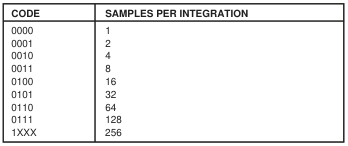
Multiple Integration Control Integrations/Conversion—L - 4 bits
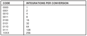
Input Range - 1 bit

Output Format - 1 bit

SECTION 7
APPLICATIONS INFORMATION
BASIC PRINTED CIRCUIT BOARD LAYOUT
As with any precision circuit, careful printed circuit layout will ensure best performance. Make short, direct interconnections and avoid stray wiring capacitance—particularly at the analog input pin. Digital signals should be kept as far from the analog input signals as possible on the PC board. Leakage currents between PC board traces can exceed the input bias current of the DDC101 if care is not taken. A circuit board “guard” pattern for the analog input pin and for the PC board trace that connects to the analog input pin is recommended. The guard pattern reduces leakage effects by surrounding the analog input pin and trace with a low impedance analog ground. Leakage currents from other
portions of the circuit will flow harmlessly to the low impedance analog ground rather than into the analog input of the DDC101. Analog ground pins are placed on either side of the analog input pin in the DDC101 package to allow convenient layout of guard patterns. Figure 22 illustrates the use of guard patterns to protect the analog input.
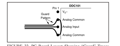
FIGURE 22. PC Board Layout Showing “Guard” Traces
Surrounding Analog Input Pin and Traces.
Power Supplies The ±5VDC supplies of the DDC101 should be bypassed with 10µF solid tantalum capacitors and 0.1µF ceramic capacitors. The supplies should each have a 10µF solid tantalum capacitor at a central point on the PC board. Each of the DDC101 power supply lines (VS+, VS–, VDD+) should have a separate 0.1µF ceramic capacitor placed as close to the DDC101 package as possible. The digital power supply voltage, VDD+ must be equal to or less than the analog power supply voltage, VS+. The analog power supply, VS+, is connected to pins 5 and 6, these pins should be hardwired together on the printed circuit board at the pins for best performance. VDD+ should be as quiet as possible with minimal noise
coupling. It is particularly important to eliminate noise from VDD+ that is non-synchronous with DDC101 operation. Figure 23 illustrates two acceptable ways to supply VDD+ power to the DDC101. The first case shows two separate +5VDC supplies for VDD+ and VS+. The second case shows the VDD+ power supply derived from the VS+ supply as used on the DDC101 Evaluation Fixture Device Under Test (DUT) board.
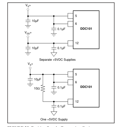
FIGURE 23. Positive Supply Connection Options.
Page 24
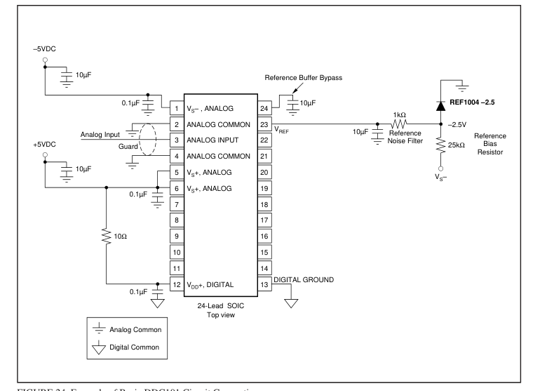
FIGURE 24. Example of Basic DDC101 Circuit Connections.
Reading Data Output Data from the previous conversion can be read any time after
the DATA VALID output is activated and before the end of
the next conversion. Data is held in an internal serial shift
register until the end of the next conversion. The data must
be completely read before the end of the next conversion or
it will be overwritten with new data. Recommended Setup The following Setup parameters are recommended, in gen-
eral, for use with the DDC101 with integration times of 1ms
or longer. Multiple integrations per conversion, where prac-
tical, will provide lowest noise as illustrated in the typical
performance curves. Measurement Time Calculation
| FUNCTION | RECOMMENDED |
| Acquisition Clocks, K Oversamples, M CDS | 16 128 Enabled |
A Continuous Integration Cycle consists of the Acquisition
Time, Initial Data Point Collection, Tracking Interval, and
Final Data Point Collection. The user can select these
functions as illustrated in Table XV.
The time between “Final Data point Start” commands is the
Integration Time, TINT. The Measurement Time, TMEAS, is the
Integration time reduced by the Acquisition Time and by the
Oversampling Time, TOS.
TMEAS = TINT - TACQ - TOS.
When CDS is used; TOS, the oversampling time, is the time
required to collect a data point (M clock periods). Each
group of samples is averaged with the result at the midpoint
of each sample group. Therefore, with CDS, TOS = M clock
periods. This is shown in Figure 25. Two calculations of the Measurement Time are shown
| FUNCTION | CLOCK CYCLES | USER CONTROLLED |
| Acquisition Time, K Initial Data Point Samples, M(1) Tracking Interval Final Data Point Samples, M(1) | 1, 16, 32 1, 2, 4, 8, 16, 32,64, 128, 256 Variable 1, 2, 4, 8, 16, 32, 64, 128, 256 | Yes Yes Yes Yes |
NOTE: (1) Will be the same in CDS mode, initial Data Point Samples = 0 in non- CDS mode.
TABLE XV. Components of Integration Cycle.
Page 25
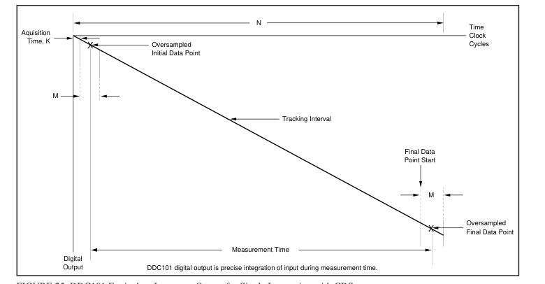
FIGURE 25. DDC101 Equivalent Integrator Output for Single Integration with CDS.
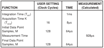
TABLE XVI. Measurement Time with CDS.
below: one with Correlated Double Sampling (CDS) and the
other without CDS. Each example assumes that the recom-
mended system clock frequency of 2MHz is used and that
the time between “Final Data point Start” commands, (the
integration time, TINT) is 1ms. Example with CDS. The Measurement Time with CDS is
calculated as the Integration Time (TINT) of 1ms less TACQ
and TOS. TOS, the oversampling time, is 1/2 of the Initial Data
Point time plus 1/2 the Final Data Point time since each
group of samples is averaged with the result at the midpoint
of each sample group. Therefore, the Measurement Time = 1ms –(8 + 32 + 32)µs
= 928µs.
Example without CDS. The Measurement Time without
CDS is calculated as the Total Integration Time (TINT) of
1ms less TACQ and TOS. TOS, the oversampling time, is 1/2 of
the Final Data Point time since this group of samples is
averaged with the result at the midpoint of the sample group. Therefore, the Measurement Time = 1ms –(0.5 + 32)µs
= 967.5µs.
| FUNCTION | USER SETTING (Clock Cycles) | TIME | MEASUREMENT (Calculated) |
| Integration Time (T ) INT Acquisition Time, K (T ) “No CDS” ACQ Initial Data Point Samples Measurement Time Final Data Point Samples, M | 1 None 128 | 1ms 0.5µs 0µs 64µs | 967.5µs |
TABLE XVII. Measurement Time without CDS.
Input Current Calculation The following formula calculates the input current from the
actual DDC output:
500pC • DDCoutput
220
With CDS:
i =
TMEAS
500pC • DDCoutput
220
i =
TINT – K clock periods – M clock periods
500pC • DDCoutput
Without CDS:
220 i =
TMEAS
500pC • DDCoutput
220
i =
TINT – K clock periods – M / 2 clock periods
Page 26
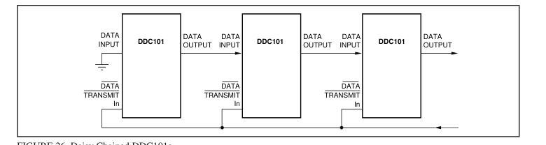
FIGURE 26. Daisy Chained DDC101s.
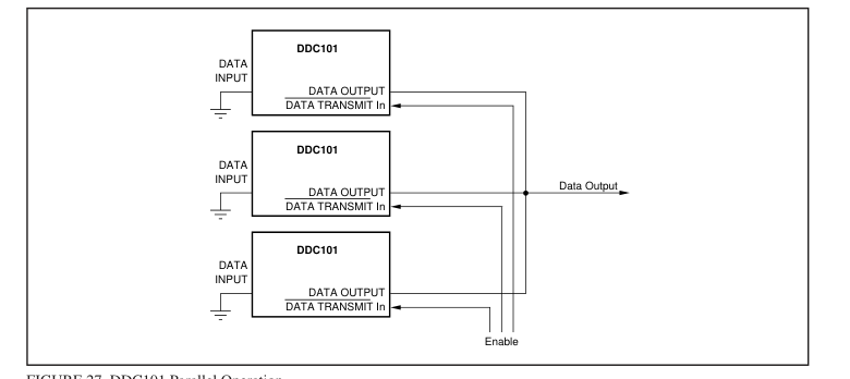
FIGURE 27. DDC101 Parallel Operation.
MULTIPLE DDC101 OPERATION
Multiple DDC101 units can be connected in serial or parallel configuration as illustrated in Figures 26 and 27. DATA OUTPUT can be used with DATA INPUT to “daisy chain” the output of several DDC101 units together to minimize wiring; in this mode of operation, the serial data output is shifted through multiple DDC101s (Figure 26). DATA OUTPUT is in a high impedance state until DATA TRANSMIT In is active. In this way, several DDC101 units can be connected in parallel to be enabled by the DATA TRANSMIT In line (Figure 27).
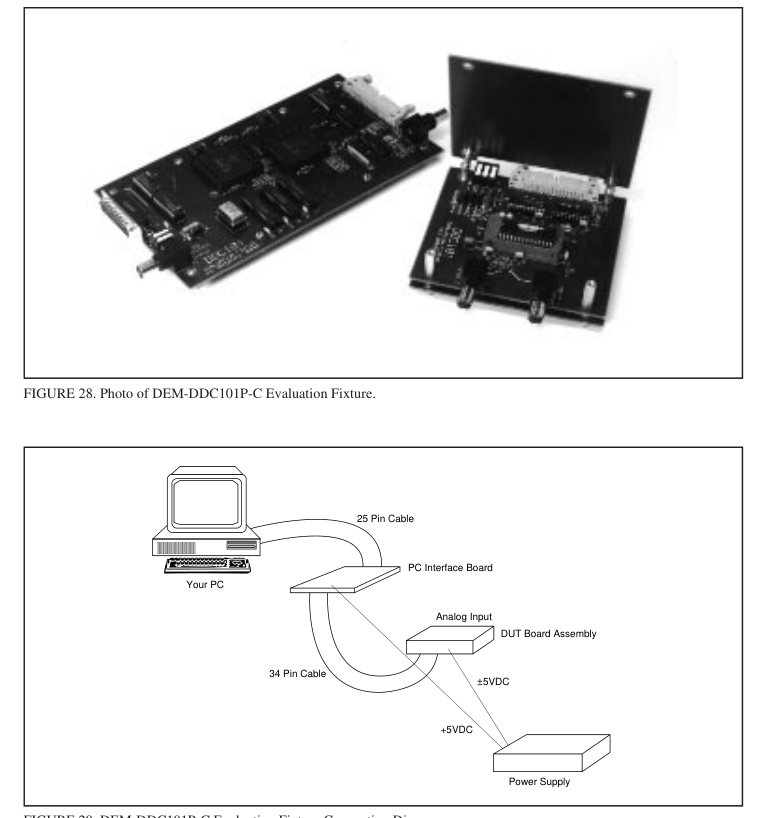
DDC101 EVALUATION FIXTURE
The DEM-DDC101P-C Evaluation Fixture is highly recommended for initial evaluation of the DDC101. It is designed for ease of use. The only additional equipment required to do
a complete evaluation of the performance of the DDC101 is an IBM compatible PC with EGA or VGA graphics, a parallel interface port, a laser printer (optional), a ±5VDC power supply, and a signal source. The DEM-DDC101P-C software is mouse compatible and retrieves data from up to 32 DDC101s in an easy to read, graphical format on the screen. The DEM-DDC101P-C Evaluation Fixture includes a PC Interface Board (with necessary parts), a DDC101 Board, a 25-pin ribbon connector and a 34-pin ribbon connector. The PC Interface Board makes timing commands and access to and from the DDC101 test board possible through the provided PC software. Data sheet, LI-439, provides complete information describing the
evaluation fixture.
Page 27