


 Download PDF
OPA2631 BURR-BROWN
Document overview
- PDF pages: 17
Technical content
Page 1
| SINGLES | DUALS | |
| Medium Speed, No Disable With Disable | OPA631 OPA632 | OPA2631 — |
| High Speed, No Disable With Disable | OPA634 OPA635 | OPA2634 — |
© 1999 Burr-Brown Corporation
PDS-1378A
Printed in U.S.A. August, 1999
Page 2
SPECIFICATIONS: VS = +5V
At TA = 25°C, G = +2, RF = 750Ω, and RL = 150Ω to VS/2, unless otherwise noted.
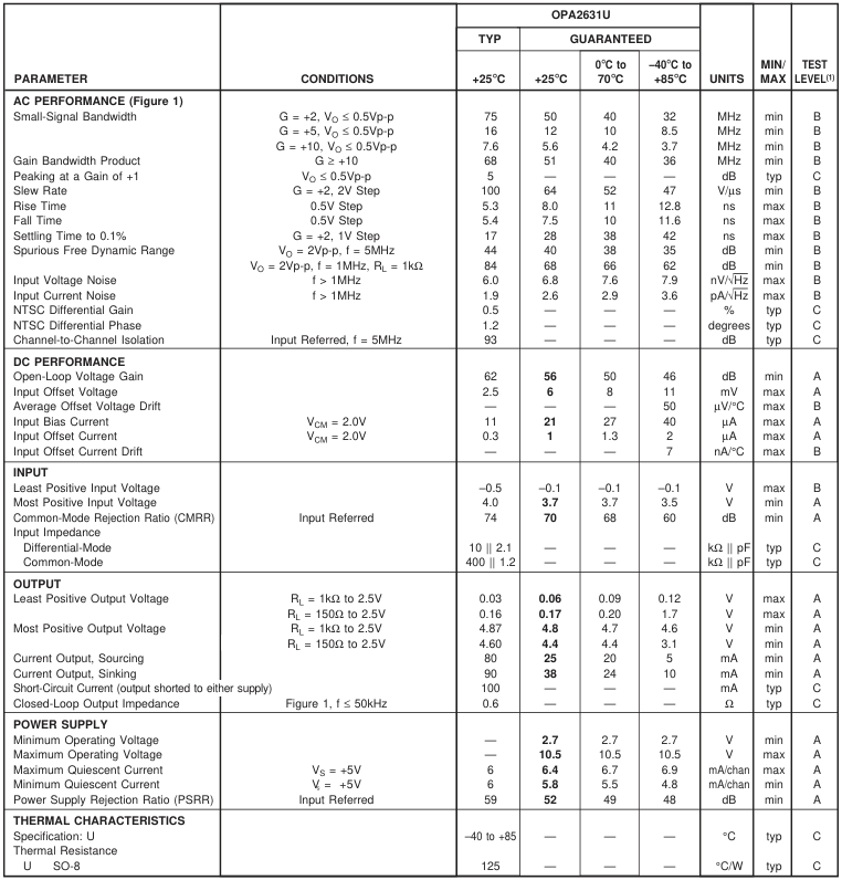
NOTE: (1) Test Levels: (A) 100% tested at 25°C. Over temperature limits by characterization and simulation. (B) Limits set by characterization and simulation. (C) Typical value only for information.
Page 3
SPECIFICATIONS: VS = +3V
At TA = 25°C, G = +2, RF = 750Ω, and RL = 150Ω to VS/2, unless otherwise noted.
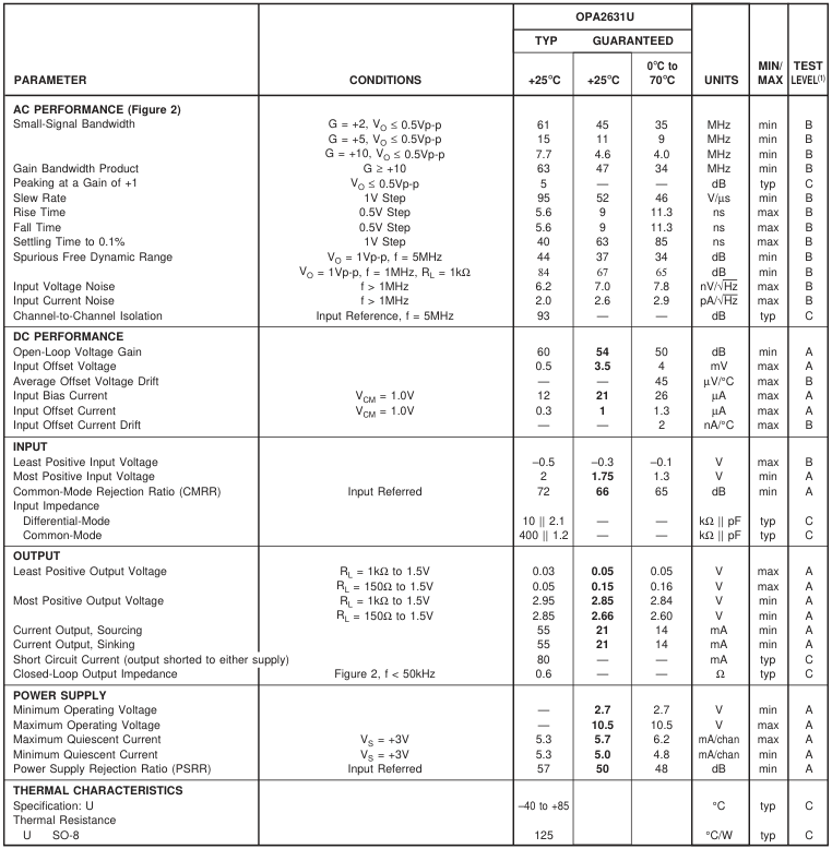
NOTE: (1) Test Levels: (A) 100% tested at 25°C. Over temperature limits by characterization and simulation. (B) Limits set by characterization and simulation. (C) Typical value only for information.
The information provided herein is believed to be reliable; however, BURR-BROWN assumes no responsibility for inaccuracies or omissions. BURR-BROWN assumes no responsibility for the use of this information, and all use of such information shall be entirely at the user’s own risk. Prices and specifications are subject to change without notice. No patent rights or licenses to any of the circuits described herein are implied or granted to any third party. BURR-BROWN does not authorize or warrant any BURR-BROWN product for use in life support devices and/or systems.
Page 4
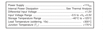
ABSOLUTE MAXIMUM RATINGS
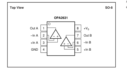
PIN CONFIGURATIONS
PACKAGE/ORDERING INFORMATION
ELECTROSTATIC
DISCHARGE SENSITIVITY
Electrostatic discharge can cause damage ranging from perfor-
mance degradation to complete device failure. Burr-Brown Corpo-
ration recommends that all integrated circuits be handled and stored
using appropriate ESD protection methods.
ESD damage can range from subtle performance degradation to
complete device failure. Precision integrated circuits may be more
susceptible to damage because very small parametric changes
could cause the device not to meet published specifications.
| PRODUCT | PACKAGE | PACKAGE DRAWING NUMBER(1) | SPECIFIED TEMPERATURE RANGE | PACKAGE MARKING | ORDERING NUMBER(2) | TRANSPORT MEDIA |
| OPA2631U " | SO-8 Surface-Mount " | 182 " | –40°C to +85°C " | OPA2631 " | OPA2631U OPA2631U/2K5 | Rails Tape and Reel |
NOTES: (1) For detailed drawing and dimension table, please see end of data sheet, or Appendix C of Burr-Brown IC Data Book. (2) Models with a slash (/) are available only in Tape and Reel in the quantities indicated (e.g., /2K5 indicates 2500 devices per reel). Ordering 2500 pieces of “OPA2631U/2K5” will get a single 2500-piece Tape and Reel. For detailed Tape and Reel mechanical information, refer to Appendix B of Burr-Brown IC Data Book.
Page 5
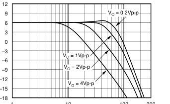
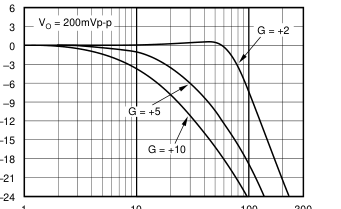
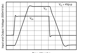
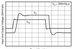
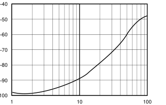
TYPICAL PERFORMANCE CURVES: VS = +5V
At TA = 25°C, G = +2, RF = 750Ω, and RL = 150Ω to VS /2, unless otherwise noted (see Figure 2).
LARGE-SIGNAL FREQUENCY RESPONSE
SMALL-SIGNAL FREQUENCY RESPONSE
1
10
100 300
1
Frequency (MHz)
SMALL-SIGNAL PULSE RESPONSE
10
100 300
Frequency (MHz)
LARGE-SIGNAL PULSE RESPONSE
Time (10ns/div)
OUTPUT SWING vs LOAD RESISTANCE
Time (10ns/div)
CHANNEL-TO-CHANNEL CROSSTALK
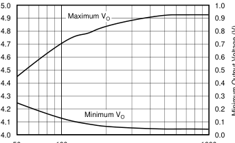
50 100
1000
Frequency (MHz)
RL (Ω)
Page 6
TYPICAL PERFORMANCE CURVES: VS = +5V (Cont.)
At TA = 25°C, G = +2, RF = 750Ω, and RL = 150Ω to VS /2, unless otherwise noted (see Figure 1).
HARMONIC DISTORTION vs OUTPUT VOLTAGE
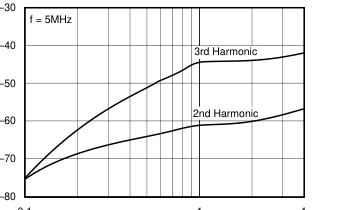
0.1
1
4
Output Voltage (Vp-p)
HARMONIC DISTORTION vs INVERTING GAIN
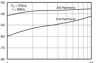
1
10
Gain Magnitude (V/V)
HARMONIC DISTORTION vs LOAD RESISTANCE
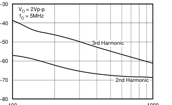
100
1000
RL (Ω)
HARMONIC DISTORTION vs NON-INVERTING GAIN
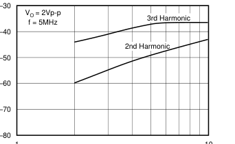
1
10
Gain Magnitude (V/V)
HARMONIC DISTORTION vs FREQUENCY
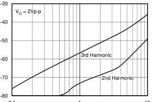
0.1
1
10
Frequency (MHz)
HARMONIC DISTORTION vs SUPPLY VOLTAGE
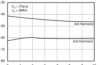
3 4 5 6 7 8 9 10
Single Supply Voltage (V)
Page 7
TYPICAL PERFORMANCE CURVES: VS = +5V (Cont.)
At TA = 25°C, G = +2, RF = 750Ω, and RL = 150Ω to VS /2, unless otherwise noted (see Figure 1).
TWO-TONE, 3rd-ORDER INTERMODULATION SPURIOUS
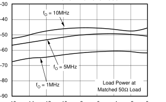
–16 –14 –12 –10 –8
–6 –4 –2 0
Single-Tone Load Power (dBm)
INPUT NOISE DENSITY vs FREQUENCY
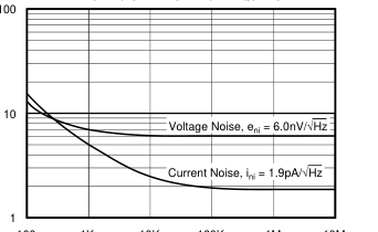
100 1K 10K 100K 1M 10M
Frequency (Hz)
FREQUENCY RESPONSE vs CAPACITIVE LOAD
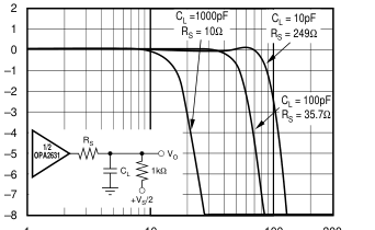
1
10
100 300
Frequency (MHz)
HARMONIC DISTORTION vs NON-INVERTING GAIN
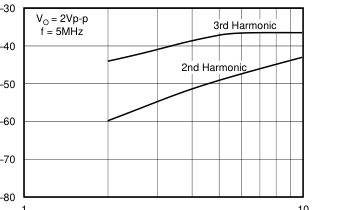
1
10
Gain Magnitude (V/V)
RECOMMENDED RS vs CAPACITIVE LOAD
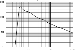
1000
1
10
100
1000
Capacitive Load (pF)
OPEN-LOOP GAIN AND PHASE
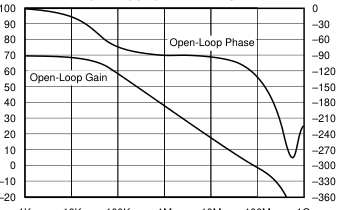
1K 10K 100K 1M 10M 100M 1G
Frequency (Hz)
Page 8
TYPICAL PERFORMANCE CURVES: VS = +5V (Cont.)
At TA = 25°C, G = +2, RF = 750Ω, and RL = 150Ω to VS /2, unless otherwise noted (see Figure 1).
CLOSED-LOOP OUTPUT IMPEDANCE vs FREQUENCY
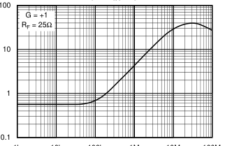
1k 10k 100k 1M 10M 100M
Frequency (Hz)
INPUT DC ERRORS vs TEMPERATURE
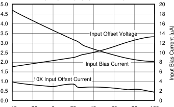
–40 –20 0 20 40 60 80 100
Temperature (°C)
POWER SUPPLY AND OUTPUT CURRENT vs TEMPERATURE
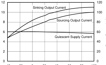
–40 –20 0 20 40 60 80 100
Temperature (°C)
Page 9
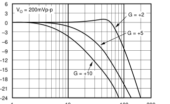
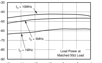
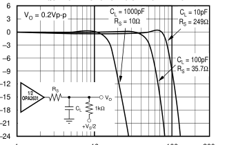
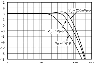
TYPICAL PERFORMANCE CURVES: VS = +3V
At TA = 25°C, G = +2, RF = 750Ω, and RL = 150Ω to VS /2, unless otherwise noted (see Figure 1).
SMALL-SIGNAL FREQUENCY RESPONSE
1
10
100 300
Frequency (MHz)
TWO-TONE, 3rd-ORDER INTERMODULATION SPURIOUS
–16 –14 –12 –10 –8 –6 –4
Single-Tone Load Power (dBm)
FREQUENCY RESPONSE vs CAPACITIVE LOAD
1
10
100 300
Frequency (MHz)
LARGE-SIGNAL FREQUENCY RESPONSE
1
10
100 300
Frequency (MHz)
RECOMMENDED RS vs CAPACITIVE LOAD
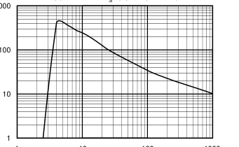
1000
1
10
100
1000
Capacitive Load (pF)
OUTPUT SWING vs LOAD RESISTANCE
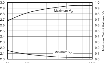
50 100
1000
RL (Ω)
Page 10
TYPICAL PERFORMANCE CURVES: VS = +3V (Cont.)
At TA = 25°C, G = +2, RF = 750Ω, and RL = 150Ω to VS /2, unless otherwise noted (see Figure 2).
SUPPLY AND OUTPUT CURRENTS vs SUPPLY VOLTAGE
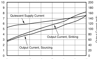
3 4 5 6 7 8 9 10
Supply Voltage (V)
SLEW RATE AND GAIN BANDWIDTH PRODUCT vs SUPPLY VOLTAGE
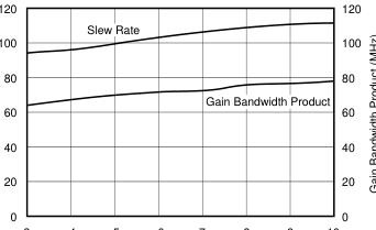
3 4 5 6 7 8 9 10
Supply Voltage (V)
Page 11
APPLICATIONS INFORMATION
WIDEBAND VOLTAGE-FEEDBACK OPERATION
The OPA2631 is a unity-gain stable, very high-speed, voltage-feedback op amp designed for single-supply operation (+3V to +5V). The input stage supports input voltages below ground, and within 1.0V of the positive supply. The complementary common-emitter output stage provides an output swing to within 30mV of ground and 130mV of the positive supply. It is compensated to provide stable operation with a wide range of resistive loads. Figure 1 shows the AC-coupled, gain of +2 configuration used for the +5V Specifications and Typical Performance Curves. For test purposes, the input impedance is set to 50Ω with a resistor to ground. Voltage swings reported in the
Specifications are taken directly at the input and output pins. For the circuit of Figure 1, the total effective load on the output at high frequencies is 150Ω || 1500Ω. The 1.50kΩ resistors at the non-inverting input provide the commonmode bias voltage. Their parallel combination equals the DC resistance at the inverting input, minimizing the output DC offset.
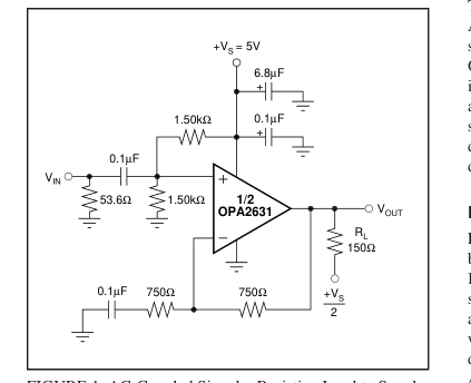
FIGURE 1. AC-Coupled Signal—Resistive Load to Supply Midpoint.
Figure 2 shows the DC-coupled, gain of +2 configuration used for the +3V Specifications and Typical Performance Curves. For test purposes, the input impedance is set to 50Ω with a resistor to ground. Though not strictly a “rail-to-rail” design, this part comes very close, while maintaining excellent performance. It will deliver ≈ 2.9Vp-p on a single +3V supply with 61MHz bandwidth. The 374Ω and 2.26kΩ resistors at the input level-shift VIN so that VOUT is within the allowed output voltage range when VIN = 0. See the Typical Performance Curves for information on driving capacitive loads.
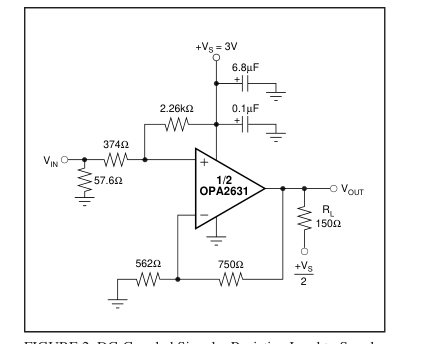
FIGURE 2. DC-Coupled Signal—Resistive Load to Supply Midpoint.
SINGLE-SUPPLY ADC CONVERTER INTERFACE
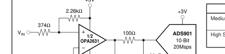
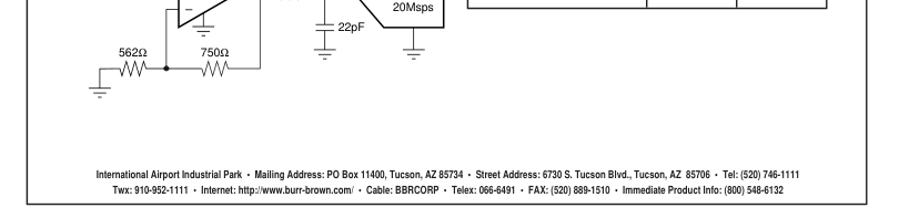
The front page shows a DC-coupled, single-supply dual ADC driver circuit. Many systems are now requiring +3V supply capability of both the ADC and its driver. The OPA2631 provides excellent performance in this demanding application. Its large input and output voltage ranges, and low distortion support converters such as the ADS901 shown in this figure. The input level-shifting circuitry was designed so that VIN can be between 0V and 0.5V, while delivering an output voltage of 1V to 2V for the ADS901.
BANDPASS FILTER
Figure 3 shows a single OPA2631 implementing a 6th-order bandpass filter. This filter cascades two 2nd-order Sallen- Key sections with transmission zeros, and a double real pole section. It has –3dB frequencies of 630kHz and 1.5MHz, and –40dB frequencies of 230kHz and 4.2MHz. This filter was designed to work well on +5V or ±5V supplies, while driving an A/D converter at 6MSPS to 10MSPS (e.g., the ADS804). The filter transfer function is based on a 4th-order elliptic bandpass filter, with real highpass and lowpass poles added at the output to give a 6th-order response. The components were chosen to give this transfer function. The 20Ω resistor isolates the first OPA2631 output from capacitive loading,
but affects the response at very high frequencies only. Figure 4 shows the nominal response simulated by SPICE®.
DC LEVEL SHIFTING
Figure 5 shows a DC-coupled non-inverting amplifier that level-shifts the input up to accommodate the desired output voltage range. Given the desired signal gain (G), and the amount VOUT needs to be shifted up (∆VOUT) when VIN is
Page 12
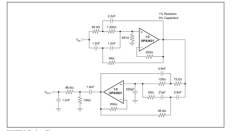
FIGURE 3. Bandpass Filter.
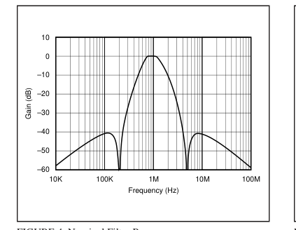
FIGURE 4. Nominal Filter Response.
at the center of its range, the following equations give the resistor values that produce the best DC offset. NG = G + ∆VOUT/VS R1 = R4/G R2 = R4/(NG – G) R3 = R4/(NG –1) where: NG = 1 + R4/R3 (Noise Gain) VOUT = (G)VIN + (NG – G)VS
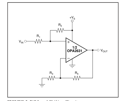
FIGURE 5. DC Level Shifting Circuit.
Make sure that VIN and VOUT stay within the specified input and output voltage ranges. The front page circuit is a good example of this type of application. It was designed to take VIN between 0V and 0.5V, and produce VOUT between 1V and 2V, when using a +3V supply. This means G = 2.00, and ∆VOUT = 1.50V – G
- 0.25V = 1.00V. Plugging into the above equations gives: NG = 2.33, R1 = 375Ω, R2 = 2.25kΩ, and R3 = 563Ω. The resistors were adjusted to the nearest standard values.
Page 13
NON-INVERTING AMPLIFIER WITH
REDUCED PEAKING
Figure 6 shows a non-inverting amplifier that reduces peaking at low gains. The resistor RC compensates the OPA2631 to have higher Noise Gain (NG), which reduces the AC response peaking (typically 5dB at G = +1 without RC) without changing the DC gain. VIN needs to be a low impedance source, such as an op amp. The resistor values are low to reduce noise. Using both RT and RF helps minimize the impact of parasitic impedances.
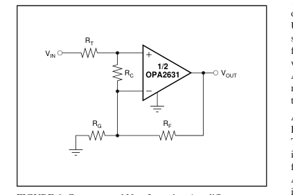
FIGURE 6. Compensated Non-Inverting Amplifier.
The Noise Gain can be calculated as follows:
RF
G1 = 1 + RG RT + RF/G1
G2 = 1 +
RC
NG = G1G2
A unity gain buffer can be designed by selecting RT = RF = 20.0Ω and RC = 40.2Ω (do not use RG). This gives a Noise Gain of 2, so its response will be similar to the Characteristics Plots with G = +2 which typically gives a flat frequency response, but with less bandwidth.
DESIGN-IN TOOLS
DEMONSTRATION BOARDS
A single PC board is available to assist in the initial evaluation of circuit performance using the OPA2631. It is available free as an unpopulated PC board delivered with descriptive documentation. The summary information for this board is shown below:
| PRODUCT | PACKAGE | BOARD PART NUMBER | LITERATURE REQUEST NUMBER |
|---|---|---|---|
| OPA2631U | 8-Pin SO-8 | DEM-OPA268xU | MKT-352 |
Contact the Burr-Brown Applications support line to request this board.
OPERATING SUGGESTIONS
OPTIMIZING RESISTOR VALUES
Since the OPA2631 is a voltage feedback op amp, a wide range of resistor values may be used for the feedback and gain setting resistors. The primary limits on these values are set by dynamic range (noise and distortion) and parasitic capacitance considerations. For a non-inverting unity gain follower application, the feedback connection should be made with a 25Ω resistor, not a direct short (see Figure 6). This will isolate the inverting input capacitance from the output pin and improve the frequency response flatness. Usually, for G > 1 application, the feedback resistor value should be between 200Ω and 1.5kΩ. Below 200Ω, the feedback network will present additional output loading
which can degrade the harmonic distortion performance. Above 1.5kΩ, the typical parasitic capacitance (approximately 0.2pF) across the feedback resistor may cause unintentional band-limiting in the amplifier response. A good rule of thumb is to target the parallel combination of RF and RG (Figure 1) to be less than approximately 400Ω. The combined impedance RF || RG interacts with the inverting input capacitance, placing an additional pole in the feedback network and thus, a zero in the forward response. Assuming a 3pF total parasitic on the inverting node, holding RF || RG <400Ω will keep this pole above 130MHz. By itself, this constraint implies that the feedback resistor RF
can increase to several kΩ at high gains. This is acceptable as long as the pole formed by RF and any parasitic capacitance appearing in parallel is kept out of the frequency range of interest.
BANDWIDTH VS GAIN: NON-INVERTING OPERATION
Voltage feedback op amps exhibit decreasing closed-loop bandwidth as the signal gain is increased. In theory, this relationship is described by the Gain Bandwidth Product (GBP) shown in the specifications. Ideally, dividing GBP by the non-inverting signal gain (also called the Noise Gain, or NG) will predict the closed-loop bandwidth. In practice, this only holds true when the phase margin approaches 90°, as it does in high gain configurations. At low gains (increased feedback factors), most amplifiers will exhibit a more complex response with lower phase margin. The OPA2631 is compensated to give a slightly peaked response in a noninverting gain of 2 (Figure 1). This results in a typical gain
of +2 bandwidth of 75MHz, far exceeding that predicted by dividing the 68MHz GBP by 2. Increasing the gain will cause the phase margin to approach 90° and the bandwidth to more closely approach the predicted value of (GBP/NG). At a gain of +10, the 7.6MHz bandwidth shown in the Typical Specifications is close to that predicted using the simple formula and the typical GBP. The OPA2631 exhibits minimal bandwidth reduction going to +3V single supply operation as compared with +5V supply. This is because the internal bias control circuitry retains nearly constant quiescent current as the total supply voltage between the supply pins is changed.
Page 14
INVERTING AMPLIFIER OPERATION
Since the OPA2631 is a general purpose, wideband voltage feedback op amp, all of the familiar op amp application circuits are available to the designer. Figure 7 shows a typical inverting configuration where the I/O impedances and signal gain from Figure 1 are retained in an inverting circuit configuration. Inverting operation is one of the more common requirements and offers several performance benefits. The inverting configuration shows improved slew rate and distortion. It also biases the input at VS/2 for the best headroom. The output voltage can be independently moved with bias adjustment resistors connected to the inverting input.
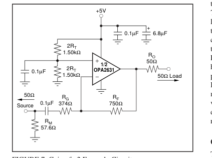
FIGURE 7. Gain of –2 Example Circuit.
In the inverting configuration, three key design consideration must be noted. The first is that the gain resistor (RG) becomes part of the signal channel input impedance. If input impedance matching is desired (which is beneficial whenever the signal is coupled through a cable, twisted pair, long PC board trace or other transmission line conductor), RG may be set equal to the required termination value and RF adjusted to give the desired gain. This is the simplest approach and results in optimum bandwidth and noise performance. However, at low inverting gains, the resultant feedback resistor value can present a significant load to the amplifier output. For an inverting gain of 2, setting RG to
50Ω for input matching eliminates the need for RM but requires a 100Ω feedback resistor. This has the interesting advantage that the noise gain becomes equal to 2 for a 50Ω source impedance—the same as the non-inverting circuits considered above. However, the amplifier output will now see the 100Ω feedback resistor in parallel with the external load. In general, the feedback resistor should be limited to the 200Ω to 1.5kΩ range. In this case, it is preferable to increase both the RF and RG values as shown in Figure 7, and then achieve the input matching impedance with a third resistor (RM) to ground. The total input impedance becomes the parallel combination of RG and RM.
The second major consideration, touched on in the previous paragraph, is that the signal source impedance becomes part of the noise gain equation and hence influences the bandwidth. For the example in Figure 7, the RM value combines in parallel with the external 50Ω source impedance, yielding an effective driving impedance of 50Ω || 576Ω = 26.8Ω. This impedance is added in series with RG for calculating the noise gain. The resultant is 2.87 for Figure 7, as opposed to only 2 if RM could be eliminated as discussed above. The bandwidth will therefore be lower for the gain of –2 circuit of Figure 7 (NG = +2.9) than for the gain of +2 circuit of Figure 1. The third important consideration in inverting amplifier
design is setting the bias current cancellation resistors on the non-inverting input (a parallel combination of RT = 750Ω). If this resistor is set equal to the total DC resistance looking out of the inverting node, the output DC error, due to the input bias currents, will be reduced to (input offset current) • RF. The inverting input's bias current flows through RF because of the 0.1µF capacitor. Thus, we need RT = 750Ω = 1.50kΩ||1.50kΩ To reduce the additional high frequency noise introduced by this RT resistor, and power supply feedthrough, it is bypassed with a capacitor. If we had RT < 400Ω, its noise contribution would be minimal. As a minimum, the OPA2631 requires an RT
value of 50Ω to damp out parasitic-induced peaking—a direct short to ground on the non-inverting input runs the risk of a very high frequency instability in the input stage.
OUTPUT CURRENT AND VOLTAGE
The OPA2631 provides outstanding output voltage capability. Under no-load conditions at +25°C, the output voltage typically swings closer than 130mV to either supply rail; the guaranteed swing limit is within 400mV of either rail (VS = +5V). The minimum specified output voltage and current specifications over temperature are set by worst-case simulations at the cold temperature extreme. Only at cold start-up will the output current and voltage decrease to the numbers shown in the guaranteed tables. As the output transistors deliver power, their junction temperatures will increase, decreasing their VBE’s (increasing the available output voltage swing) and
increasing their current gains (increasing the available output current). In steady-state operation, the available output voltage and current will always be greater than that shown in the over-temperature specifications since the output stage junction temperatures will be higher than the minimum specified operating ambient. To maintain maximum output stage linearity, no output short-circuit protection is provided. This will not normally be a problem since most applications include a series matching resistor at the output that will limit the internal power dissipation if the output side of this resistor is shorted to ground.
Page 15
DRIVING CAPACITIVE LOADS
One of the most demanding and yet very common load conditions for an op amp is capacitive loading. Often, the capacitive load is the input of an A/D converter—including additional external capacitance which may be recommended to improve A/D linearity. A high speed, high open-loop gain amplifier like the OPA2631 can be very susceptible to decreased stability and closed-loop response peaking when a capacitive load is placed directly on the output pin. When the primary considerations are frequency response flatness, pulse response fidelity and/or distortion, the simplest and most effective solution is to isolate the capacitive load from the feedback loop by inserting a series isolation resistor
between the amplifier output and the capacitive load. The Typical Performance Curves show the recommended RS versus capacitive load and the resulting frequency re- sponse at the load. Parasitic capacitive loads greater than 2pF can begin to degrade the performance of the OPA2631. Long PC board traces, unmatched cables, and connections to multiple devices can easily exceed this value. Always consider this effect carefully, and add the recommended series resistor as close as possible to the output pin (see Board Layout Guidelines). The criterion for setting this RS resistor is a maximum bandwidth, flat frequency response at the load. For a gain of +2, the frequency response at the output pin is already
slightly peaked without the capacitive load, requiring relatively high values of RS to flatten the response at the load. Increasing the noise gain will also reduce the peaking (see Figure 6).
DISTORTION PERFORMANCE
The OPA2631 provides good distortion performance into a 150Ω load. Relative to alternative solutions, it provides exceptional performance into lighter loads and/or operating on a single +3V supply. Generally, the 3rd harmonic will dominate the distortion. Focusing then on the 3rd harmonic, increasing the load impedance improves distortion directly.
The total output spot noise voltage can be computed as the square root of the sum of all squared output noise voltage contributors. Equation 1 shows the general form for the output noise voltage using the terms shown in Figure 8.
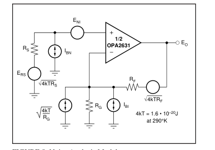
FIGURE 8. Noise Analysis Model.
Equation 1:
(
)NG2 + IBIRF
ENI2 + IBNRS 2 + 4kTRS
2 + 4kTRFNG
( )
( )
EO =
Dividing this expression by the noise gain (NG = (1+RF/RG)) will give the equivalent input-referred spot noise voltage at the non-inverting input, as shown in Equation 2. Equation 2:
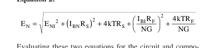
Evaluating these two equations for the circuit and component values shown in Figure 1 will give a total output spot
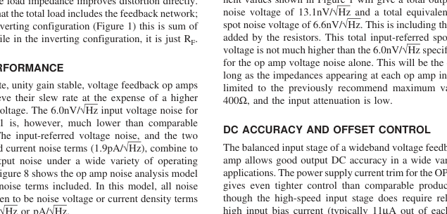
NOISE PERFORMANCE
in either nV/√Hz or pA/√Hz.
terminal), the close matching between them may be used to
Page 16
reduce the output DC error caused by this current. This is done by matching the DC source resistances appearing at the two inputs. Evaluating the configuration of Figure 1 (which has matched DC input resistances), using worst-case +25°C input offset voltage and current specifications, gives a worstcase output offset voltage equal to: (NG = non-inverting signal gain at DC) ±(NG • VOS(MAX)) ± (RF • IOS(MAX)) = ±(1 • 6.0mV) ± (750Ω • 2.0µA) = ±6.8mV = Output Offset Range for Figure 1 A fine scale output offset null, or DC operating point adjustment, is often required. Numerous techniques are available for introducing DC offset control into an op amp circuit. Most of these techniques are based on adding a DC
current through the feedback resistor. In selecting an offset trim method, one key consideration is the impact on the desired signal path frequency response. If the signal path is intended to be non-inverting, the offset control is best applied as an inverting summing signal to avoid interaction with the signal source. If the signal path is intended to be inverting, applying the offset control to the non-inverting input may be considered. Bring the DC offsetting current into the inverting input node through resistor values that are much larger than the signal path resistors. This will insure that the adjustment circuit has minimal effect on the loop gain and hence the frequency response.
THERMAL ANALYSIS
Maximum desired junction temperature will set the maximum allowed internal power dissipation as described below. In no case should the maximum junction temperature be allowed to exceed 175°C. Operating junction temperature (TJ) is given by TA + PD•θJA. The total internal power dissipation (PD) is the sum of quiescent power (PDQ) and additional power dissipated in the output stage (PDL) to deliver load power. Quiescent power is simply the specified no-load supply current times the total supply voltage across the part. PDL will depend on the required output signal and load but would, for resistive load connected to mid-supply (VS/2), be at a maximum when the
output is fixed at a voltage equal to VS/4 or 3VS/4. Under this condition, PDL = VS2/(16 • RL), where RL includes feedback network loading. Note that it is the power in the output stage and not into the load that determines internal power dissipation. As a worst-case example, compute the maximum TJ using the circuit of Figure 1 operating at the maximum specified ambient temperature of +85°C and driving a 150Ω load at mid-supply, for both channels: PD = 2 (10V • 6.9mA + 52/(16 • (150Ω || 1500Ω))) = 160mW Maximum TJ = +85°C + (0.16W • 150°C/W) = 109°C. Although this is still well below the specified maximum junction temperature, system reliability considerations may
require lower guaranteed junction temperatures. The highest
possible internal dissipation will occur if the load requires current to be forced into the output at high output voltages or sourced from the output at low output voltages. This puts a high current through a large internal voltage drop in the output transistors.
BOARD LAYOUT GUIDELINES
Achieving optimum performance with a high frequency amplifier like the OPA2631 requires careful attention to board layout parasitics and external component types. Recommendations that will optimize performance include: a) Minimize parasitic capacitance to any AC ground for all of the signal I/O pins. Parasitic capacitance on the output and inverting input pins can cause instability: on the noninverting input, it can react with the source impedance to cause unintentional bandlimiting. To reduce unwanted ca- pacitance, a window around the signal I/O pins should be opened in all of the ground and power planes around those pins. Otherwise, ground and power planes should be unbro-
ken elsewhere on the board. b) Minimize the distance (<0.25") from the power supply pins to high frequency 0.1µF decoupling capacitors. At the device pins, the ground and power plane layout should not be in close proximity to the signal I/O pins. Avoid narrow power and ground traces to minimize inductance between the pins and the decoupling capacitors. The power supply connections should always be decoupled with these capacitors. An optional supply decoupling capacitor (0.1µF) across the two power supplies (for bipolar operation) will improve 2nd harmonic distortion performance. Larger (2.2µF to 6.8µF) decoupling capacitors, effective at lower frequency,
should also be used on the main supply pins. These may be placed somewhat farther from the device and may be shared among several devices in the same area of the PC board. c) Careful selection and placement of external components will preserve the high frequency performance. Resistors should be a very low reactance type. Surfacemount resistors work best and allow a tighter overall layout. Metal film or carbon composition axially-leaded resistors can also provide good high frequency performance. Again, keep their leads and PC board traces as short as possible. Never use wirewound type resistors in a high frequency application. Since the output pin and inverting input pin are
the most sensitive to parasitic capacitance, always position the feedback and series output resistor, if any, as close as possible to the output pin. Other network components, such as non-inverting input termination resistors, should also be placed close to the package. Where double-side component mounting is allowed, place the feedback resistor directly under the package on the other side of the board between the output and inverting input pins. Even with a low parasitic capacitance shunting the external resistors, excessively high resistor values can create significant time constants that can degrade performance. Good axial metal film or surfacemount resistors have approximately 0.2pF in shunt with the
resistor. For resistor values > 1.5kΩ, this parasitic capaci-
Page 17
tance can add a pole and/or zero below 500MHz that can effect circuit operation. Keep resistor values as low as possible consistent with load driving considerations. The 750Ω feedback used in the typical performance specifications is a good starting point for design. See Figure 6 for the unity gain follower application. d) Connections to other wideband devices on the board may be made with short direct traces or through on-board transmission lines. For short connections, consider the trace and the input to the next device as a lumped capacitive load. Relatively wide traces (50mils to 100mils) should be used, preferably with ground and power planes opened up around
them. Estimate the total capacitive load and set RS from the plot of Recommended RS vs Capacitive Load. Low parasitic capacitive loads (< 5pF) may not need an RS since the OPA2631 is nominally compensated to operate with a 2pF parasitic load. Higher parasitic capacitive loads without an RS are allowed as the signal gain increases (increasing the unloaded phase margin) If a long trace is required, and the 6dB signal loss intrinsic to a doubly terminated transmission line is acceptable, implement a matched impedance transmission line using microstrip or stripline techniques (consult an ECL design handbook for microstrip and stripline layout techniques). A 50Ω environment is normally not necessary
on board, and in fact, a higher impedance environment will improve distortion as shown in the distortion versus load plots. With a characteristic board trace impedance defined (based on board material and trace dimensions), a matching series resistor into the trace from the output of the OPA2631 is used as well as a terminating shunt resistor at the input of the destination device. Remember also that the terminating impedance will be the parallel combination of the shunt resistor and the input impedance of the destination device; this total effective impedance should be set to match the trace impedance. If the 6dB attenuation of a doubly terminated transmission line is unacceptable, a long trace can be
series-terminated at the source end only. Treat the trace as a capacitive load in this case and set the series resistor value as shown in the plot of Recommended RS vs Capacitive Load. This will not preserve signal integrity as well as a
doubly terminated line. If the input impedance of the destination device is low, there will be some signal attenuation due to the voltage divider formed by the series output into the terminating impedance. e) Socketing a high speed part is not recommended. The additional lead length and pin-to-pin capacitance introduced by the socket can create an extremely troublesome parasitic network which can make it almost impossible to achieve a smooth, stable frequency response. Best results are obtained by soldering the OPA2631 onto the board.
INPUT AND ESD PROTECTION
The OPA2631 is built using a very high speed complementary bipolar process. The internal junction breakdown voltages are relatively low for this very small geometry device. This breakdown is reflected in the Absolute Maximum Ratings table. All device pins are protected with internal ESD protection diodes to the power supplies as shown in Figure 9. These diodes provide moderate protection to input overdrive voltages above the supplies as well. The protection diodes can typically support 30mA continuous current. Where higher currents are possible (e.g., in systems with ±15V supply parts driving into the OPA2631), current-limiting series resistors should be added into the two inputs. Keep these
resistor values as low as possible since high values degrade both noise performance and frequency response.
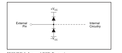
FIGURE 9. Internal ESD Protection.